AI: A Technical History

Introduction

I enjoyed learning about the history of machine learning and the computational methods that led to artificial intelligence. I came to it as a physician, so I keep pulling the story back toward medicine - what a diagnosis has in common with a classification boundary, and where these systems might actually help at the bedside. I’ve tried to take some of that and put it into a timeline to help me appreciate and understand it. Hope anyone reading this enjoys walking through it as well.

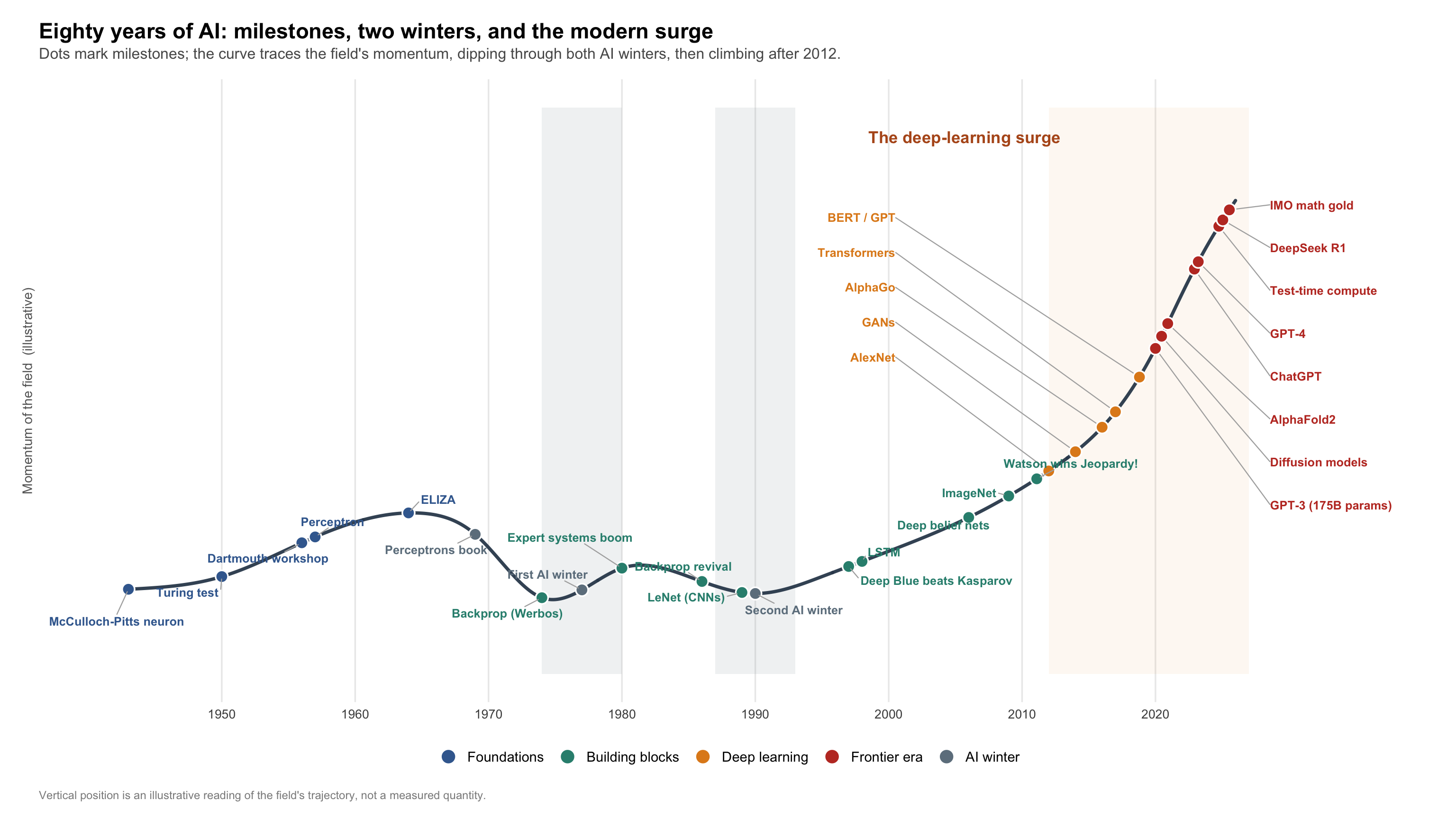
The timeline shows how AI development has clustered - long quiet periods followed by rapid advances, most of them concentrated in the last decade.

The Complete AI Timeline

Eighty years of breakthroughs, winters, and revolutions - scroll through, or skim the Significance column for the hinge points.

Era	Year	Breakthrough	Key People	Impact	Significance
Foundations	1943	McCulloch-Pitts Neuron	McCulloch & Pitts	First mathematical neuron	▲Paradigm Shift
Foundations	1948	Information Theory	Claude Shannon	Information becomes measurable	◆Major Advance
Foundations	1949	Hebbian Learning	Donald Hebb	Learning as synaptic strengthening	●Important
Foundations	1950	Turing Test	Alan Turing	Intelligence judged by behavior	◆Major Advance
Foundations	1956	Dartmouth Conference	McCarthy & Minsky	AI named and founded	▲Paradigm Shift
Foundations	1957	Perceptron	Frank Rosenblatt	First machine that learns	◆Major Advance
Foundations	1957	Dynamic Programming	Richard Bellman	The recursive value function behind RL	◆Major Advance
Foundations	1959	Machine Learning Coined	Arthur Samuel	Programs improve with experience	●Important
Foundations	1966	ELIZA	Joseph Weizenbaum	First chatbot fools users	○Notable
Foundations	1966	ALPAC Report	-	Machine translation funding cut	▼Winter/Setback
Foundations	1969	Perceptrons Book	Minsky & Papert	XOR limit triggers winter	▼Winter/Setback
First Winter	1973	Lighthill Report	James Lighthill	UK cuts AI funding	▼Winter/Setback
First Winter	1974	Backprop (Thesis)	Paul Werbos	Invented but ignored	●Important
First Winter	1975	MYCIN	Edward Shortliffe	Expert-level on narrow medicine	○Notable
First Winter	1976	Statistical Speech Recognition	Jelinek, Bahl, Mercer, Baker	Language as a noisy channel, learned from data	◆Major Advance
First Winter	1979	Stanford Cart	Hans Moravec	Self-driving, one meter per five minutes	−Minor
Revival	1980	Neocognitron	Kunihiko Fukushima	CNN blueprint, a decade early	●Important
Revival	1980	Expert Systems Boom	-	AI's first commercial boom	○Notable
Revival	1982	Hopfield Networks	John Hopfield	Networks as associative memory	○Notable
Revival	1985	NetTalk	Terry Sejnowski	A network learns to read aloud	○Notable
Revival	1986	Backprop Rediscovered	Rumelhart, Hinton, Williams	Multi-layer nets finally trainable	▲Paradigm Shift
Revival	1987	Second AI Winter	-	Expert systems collapse	▼Winter/Setback
Revival	1988	Bayesian Networks	Judea Pearl	Principled reasoning under uncertainty	◆Major Advance
Revival	1989	LeNet (CNN)	Yann LeCun	CNNs read handwriting at scale	◆Major Advance
Revival	1989	Universal Approximation	Cybenko; Hornik et al.	One hidden layer can represent anything	◆Major Advance
Revival	1989	Q-Learning	Chris Watkins	Optimal control with no model of the world	◆Major Advance
Statistical ML	1990	Recurrent Networks	Jeffrey Elman	Networks gain sequence memory	●Important
Statistical ML	1992	TD-Gammon	Gerald Tesauro	Self-play RL masters backgammon	●Important
Statistical ML	1995	Support Vector Machines	Cortes & Vapnik	Principled max-margin classification	◆Major Advance
Statistical ML	1997	LSTM	Hochreiter & Schmidhuber	Memory that survives long sequences	▲Paradigm Shift
Statistical ML	1997	Deep Blue beats Kasparov	IBM	World chess champion defeated	◆Major Advance
Statistical ML	2001	Random Forests	Leo Breiman	Many random trees beat one	●Important
Statistical ML	2003	Neural Language Model	Bengio et al.	The learned word embedding, a decade early	◆Major Advance
Statistical ML	2006	Deep Belief Networks	Geoffrey Hinton	Pretraining revives deep nets	◆Major Advance
Statistical ML	2007	CUDA	NVIDIA	GPUs open to general compute	●Important
Statistical ML	2009	ImageNet Dataset	Fei-Fei Li	14M labels make scale possible	▲Paradigm Shift
Statistical ML	2010	ReLU Activation	Nair & Hinton	Gradients survive depth	◆Major Advance
Deep Learning	2012	AlexNet	Krizhevsky et al.	ImageNet error nearly halved	▲Paradigm Shift
Deep Learning	2013	DQN (Atari)	DeepMind	Reinforcement learning from raw pixels	◆Major Advance
Deep Learning	2013	Word2Vec	Tomas Mikolov	Meaning becomes geometry	●Important
Deep Learning	2014	GANs	Ian Goodfellow	Two networks compete, images emerge	◆Major Advance
Deep Learning	2014	Attention (Translation)	Bahdanau, Cho, Bengio	Attention invented for translation	◆Major Advance
Deep Learning	2014	VGGNet	Oxford	Depth from simple 3x3 filters	○Notable
Deep Learning	2014	Sequence-to-Sequence	Sutskever, Vinyals, Le	Any sequence in, any sequence out	◆Major Advance
Deep Learning	2015	ResNet	Kaiming He	Skip connections unlock 152 layers	◆Major Advance
Deep Learning	2015	Batch Normalization	Ioffe & Szegedy	Deep training becomes reliable	●Important
Deep Learning	2016	AlphaGo beats Lee Sedol	DeepMind	Go falls a decade early	▲Paradigm Shift
Deep Learning	2016	Neural Machine Translation	Google	End-to-end translation deployed	●Important
Deep Learning	2016	Diabetic Retinopathy Screening	Gulshan, Peng et al.	Matches the ophthalmologist reference standard	◆Major Advance
Transformer Era	2017	Transformer	Vaswani et al.	Attention replaces recurrence	▲Paradigm Shift
Transformer Era	2018	BERT	Google	Pretrain once, fine-tune everywhere	◆Major Advance
Transformer Era	2018	GPT-1	OpenAI	Generative pretraining shows promise	●Important
Transformer Era	2018	IDx-DR (FDA Authorized)	Michael Abramoff	First diagnosis with no physician reading it	◆Major Advance
Transformer Era	2019	GPT-2	OpenAI	Fluency prompts a staged release	●Important
Transformer Era	2019	Clinical Algorithmic Bias	Obermeyer et al.	Well-calibrated and clinically unjust at once	●Important
Transformer Era	2020	GPT-3	OpenAI	Scale alone yields new abilities	▲Paradigm Shift
Transformer Era	2020	Scaling Laws	Kaplan et al.	Loss falls predictably with scale	◆Major Advance
Transformer Era	2020	Diffusion Models (DDPM)	Ho, Jain, Abbeel	Generation by reversing noise, beating GANs	▲Paradigm Shift
Transformer Era	2020	Vision Transformer	Dosovitskiy et al.	Convolution turns out to be optional	◆Major Advance
Transformer Era	2020	Halicin Antibiotic	Stokes, Barzilay, Collins	AI proposes molecules, not just reads data	●Important
Transformer Era	2021	CLIP	OpenAI	Images and text share one space	◆Major Advance
Transformer Era	2021	AlphaFold 2	DeepMind	Protein folding effectively solved	▲Paradigm Shift
Transformer Era	2022	InstructGPT (RLHF)	OpenAI	Models tuned to human preference	◆Major Advance
Transformer Era	2022	Stable Diffusion	Stability AI	Image generation for everyone	◆Major Advance
Transformer Era	2022	ChatGPT	OpenAI	100M users in two months	▲Paradigm Shift
Transformer Era	2022	Chain-of-Thought Prompting	Wei, Zhou, Le et al.	Reasoning elicited by prompting alone	▲Paradigm Shift
Transformer Era	2022	Chinchilla Scaling	Hoffmann, Borgeaud, Sifre	Big models were badly undertrained	◆Major Advance
Transformer Era	2023	GPT-4	OpenAI	Professional-exam-level competence	▲Paradigm Shift
Transformer Era	2023	Llama 2	Meta	Frontier-class weights, free to build on	◆Major Advance
Transformer Era	2024	Sora	OpenAI	Minute-long coherent video	●Important
Transformer Era	2024	Claude 3	Anthropic	Alignment by explicit principles	◆Major Advance
Transformer Era	2024	o1	OpenAI	Thinking longer becomes a scaling axis	◆Major Advance
Transformer Era	2024	o3	OpenAI	Reasoning crosses the ARC-AGI bar	▲Paradigm Shift
Reasoning & Agents	2025	DeepSeek R1	DeepSeek-AI	Reasoning learned by RL, in open weights	▲Paradigm Shift
Reasoning & Agents	2025	Operator & Deep Research	OpenAI (and others)	Autonomous web-browsing agents	◆Major Advance
Reasoning & Agents	2025	Gemini 2.5 Pro	Google DeepMind	Reasoning with million-token context	◆Major Advance
Reasoning & Agents	2025	Claude Opus 4 / Sonnet 4	Anthropic	Long-horizon autonomous coding	◆Major Advance
Reasoning & Agents	2025	IMO Gold-Level Reasoning	Google DeepMind (officially graded)	Olympiad gold from natural-language proofs	▲Paradigm Shift
Reasoning & Agents	2025	GPT-5	OpenAI	Unified model with reasoning router	◆Major Advance
Reasoning & Agents	2025	Grok 4	xAI	Frontier model with native tools	●Important
Reasoning & Agents	2025	Llama 4	Meta	Open-weight multimodal MoE	●Important
Reasoning & Agents	2025	Gemini 3	Google DeepMind	Record multimodal benchmark scores	◆Major Advance
Reasoning & Agents	2025	Task-Length Time Horizons	METR (Kwa, West, Becker)	Autonomy measured in task length, not score	◆Major Advance
Reasoning & Agents	2025	AlphaEvolve	Google DeepMind	The verifier is what makes discovery reliable	◆Major Advance
Reasoning & Agents	2025	Autonomous Cyber-Espionage	Reported by Anthropic	Agentic harm at scale, disputed in scope	●Important
Reasoning & Agents	2026	Claude Opus 4.6 / 4.7	Anthropic	Sustained multi-file coding agents	●Important
Reasoning & Agents	2026	GPT-5.5	OpenAI	Broad agentic knowledge-work model	●Important
Reasoning & Agents	2026	Erdos Conjecture Disproved	Lijie Chen with an OpenAI model	A model produces the counterexample, humans verify	◆Major Advance
Reasoning & Agents	2026	AI Co-Scientist	Google DeepMind	Machine hypotheses confirmed at the bench	◆Major Advance

Every video, in order

Every video on this page, in the order I would watch them if you just want the whole thing in one place. It runs roughly the way the essay does: what a network is, how it learns, the math and statistics sitting underneath, the methods that beat neural nets for a decade, then vision, sequences, attention, how LLMs are actually trained, and the generative era. Every section below also has its own shelf, repeating the relevant few in context next to the part of the story they belong to.

Part I: Thinking as Computation (1843-1969)

Where we areA century of argument. Logicians, engineers, and biologists build the case that thinking is mechanical, and the first machine that learns from examples arrives. A puzzle called exclusive-or then halts it.

Ada Lovelace and the Idea of Symbolic Computation (1843)

To understand artificial intelligence, we need to start with a fundamental question: what is computation? For most of human history, calculation meant arithmetic - adding, subtracting, manipulating numbers. The word “computer” itself referred to human beings, often women, who performed calculations by hand in astronomy observatories and ballistics labs. But in 1843, a young woman named Ada Lovelace saw something that would take humanity another century to fully appreciate: computation wasn’t about numbers at all. It was about patterns and transformations.

Lovelace was translating a French article about Charles Babbage’s Analytical Engine, a mechanical computer designed but never built. To appreciate the audacity of this machine, consider that it was conceived in the age of steam engines and gas lamps, decades before the electric light bulb. The Engine was revolutionary for its time - it had a “mill” (what we’d now call a CPU), a “store” (memory with a capacity of 1,000 50-digit numbers), and could be programmed with punched cards borrowed from the Jacquard loom. But everyone, including Babbage himself, saw it as a very sophisticated calculator. The phrase “thinking machine” actually came from Lady Byron, Ada’s mother, who saw an early Babbage engine demonstrated in 1833; but even that meant only reckoning with numbers, nothing more.

Lovelace’s notes, which she labeled A through G, ended up being three times longer than the original article. She worked on them for nine months, corresponding extensively with Babbage, who called her “the Enchantress of Numbers.” In Note G, she laid out an algorithm for calculating Bernoulli numbers - a sequence important in number theory. This algorithm, with its loops and conditional branches, is considered the first computer program. She even included what we’d now recognize as a trace table, showing the machine’s state at each step of execution. She had invented debugging before there were bugs to debug. But that’s not why she matters to AI.

The crucial insight came in Note G, where she articulated what philosophers now call the “Lovelace objection” to machine intelligence. She wrote: “The Analytical Engine has no pretensions whatever to originate anything. It can do whatever we know how to order it to perform. It can follow analysis; but it has no power of anticipating any analytical relations or truths.” This seems like a limitation - and indeed, Alan Turing would spend considerable time addressing this very objection a century later. Elsewhere in the notes she offered a vision that went far beyond her time: “Supposing, for instance, that the fundamental relations of pitched sounds in the science of harmony and of musical composition were susceptible of such expression and adaptations, the engine might compose elaborate and scientific pieces of music of any degree of complexity or extent.”

Pause and consider what she’s suggesting here. In 1843, when the most complex machines were pocket watches and steam engines, she imagined a device composing symphonies. Not playing music from a preset pattern like a music box, but creating new compositions based on encoded rules of harmony. She saw that creativity itself might be computational.

Music isn’t numbers, but it can be represented by numbers - frequencies, durations, intervals. A middle C is 261.63 Hz, an octave higher is exactly double. The pleasing sound of a major chord comes from simple frequency ratios: 4:5:6. Once represented symbolically, these relationships can be manipulated computationally. She understood that the Engine could work with any symbols whose relationships could be formally expressed - what we now call “substrate independence.” This is the birth of an idea that would take a century to realize: intelligence might be symbol manipulation. Thought might be computation.

Read in hindsight, one line even seems to prefigure machine learning: the Engine, she wrote, might act upon “any objects whose mutual fundamental relations could be expressed by those of the abstract science of operations.” She was making a point about symbolic generality rather than about learning - but it is the same intuition the rest of this history runs on. Once you can represent knowledge symbolically, you can transform it, combine it, and potentially discover something new.

In modern genomics, we see Lovelace’s principle everywhere. DNA isn’t inherently digital - it’s a physical molecule, a sugar-phosphate backbone with nucleotide bases attached. But we represent it as sequences of A, T, G, and C. Once digitized, we can compute on it - finding patterns across billions of base pairs, predicting protein folding from sequence alone, identifying disease variants among the three billion letters of the human genome. Machine learning can even decode the “grammar” of gene regulation, understanding how cells read and interpret genetic instructions. Lovelace saw this possibility when “computer” still meant a person who calculated by hand, when the idea of encoding biological information was pure fantasy.

McCulloch-Pitts: The Brain as a Logic Machine (1943)

A century after Lovelace, the question remained: how does thinking actually work? The year was 1943, and while the world was consumed by war, two researchers at the University of Chicago were working on the mystery of the mind. Their answer would launch the field of artificial neural networks.

Warren McCulloch was a neurophysiologist with the soul of a philosopher. He had trained in psychology, philosophy, and medicine, earning his MD from Columbia. But his real obsession was understanding how the wet, biological matter of the brain could give rise to logic, reasoning, and consciousness. He had spent years studying the brain’s structure, mapping neural pathways with the primitive tools of the 1940s - silver staining, light microscopy, and endless patience. He knew that neurons were cells that received electrical signals from other neurons through connections called synapses. When enough signal accumulated, the neuron would “fire,” sending its own signal forward like a biological relay switch. But how did this create thought? How could meat think?

Walter Pitts was a mathematical prodigy with an unusual and tragic background. Much of what we know about his early life comes through friends and later retellings, and some of it has surely been polished in the telling - but the outline is consistent across sources. At 12, he had run away from home to escape an abusive father and spent three days hiding in a library, where he discovered Russell and Whitehead’s Principia Mathematica. Instead of comic books or adventure stories, this homeless child read all three volumes cover to cover - a work on the foundations of mathematics so dense that most PhD students find it impenetrable. He found errors in it and wrote to Russell with corrections. At 15, still homeless and living in Chicago, he would sneak into Russell’s lectures at the University of Chicago, sitting in the back row, taking notes on scraps of paper. Russell was so impressed when they finally met that he invited Pitts to study with him at Cambridge, though Pitts was too young and too poor to accept. Instead, Pitts lived in the university’s steam tunnels, emerging for lectures and seminars like a mathematical phantom.

McCulloch and Pitts met through their mutual interest in how the brain computes. The 42-year-old physician and the 20-year-old homeless genius formed an unlikely partnership. McCulloch would later say that Pitts was the greatest genius he ever knew. They would work through the night in McCulloch’s home, with McCulloch’s wife Rook feeding them and trying to convince Pitts to sleep in a bed instead of on the floor. Their collaboration produced a 1943 paper with an unwieldy title: “A Logical Calculus of Ideas Immanent in Nervous Activity.” But the idea was elegant, even beautiful in its simplicity.

They proposed that neurons could be modeled as simple logical units, stripping away all the messy biology to reveal the computational essence. Their model was audaciously reductionist: forget about neurotransmitters, ion channels, and the hundred types of neurons in the brain. Instead, imagine each neuron as a simple decision-maker that follows three rules. First, it receives inputs from other neurons, like votes in an election. Second, each input has a weight - positive for excitatory inputs (“yes” votes), negative for inhibitory inputs (“veto” votes). Third, the neuron sums all these weighted votes, and if the total exceeds a threshold, the neuron fires its own signal forward.

In mathematical terms, this became a single inequality: Output = 1 if Σ(weight × input) > threshold, else 0. It’s a democracy of neurons, where each cell votes on whether the next should fire.

This seems almost trivially simple - so simple that some dismissed it as a toy model. But McCulloch and Pitts proved something profound using the mathematical tools of their time: networks of these simple units could compute any logical function that could be computed at all. You could build AND gates (fire only if all inputs fire), OR gates (fire if any input fires), NOT gates (fire if input doesn’t fire). They showed explicit constructions: two neurons with carefully chosen weights could implement any Boolean function. String enough together, and you could build any circuit. And if you could build any circuit, you could build a computer. The brain might be a biological implementation of a universal computing machine.

If thought was computation, and computation could be mechanized, then perhaps machines could think. They had reduced the ineffable quality of mind to binary decisions and weighted connections.

But there was a deeper implication that connected their work to the foundations of computer science itself. In 1936, Alan Turing had proven that his abstract “Turing machines” could compute any function that could be computed - a result so fundamental it defined what we mean by “computable.” Now McCulloch and Pitts showed that networks of their idealized neurons could implement any logical function - and that, granted unbounded memory, they could match the power of Turing’s machines. The equivalence was intoxicating: circuits of simplified neurons and abstract computing machines seemed to speak the same language, and (presumably) the brain spoke it too.

This meant three important things. First, the brain might be a computer in Turing’s formal sense - not metaphorically, but literally, a physical implementation of a universal computing machine. Second, we might be able to build artificial brains from non-biological components, since what mattered was the computation, not the substrate. Third, and most radically, thinking itself might be computation - not like computation, but actually computation, in the same way that heat is molecular motion, not merely like molecular motion.

But there was a crucial limitation in their model: the weights and thresholds were fixed, hardwired like a circuit board. The network couldn’t learn. It was like having a brain that was fully formed at birth, unable to adapt or improve from experience. This was particularly ironic, since the human brain’s defining characteristic is its plasticity - children learn languages effortlessly, we form new memories daily, and stroke patients can rewire their brains to recover lost functions. McCulloch and Pitts had captured the brain’s logic but not its ability to change.

In clinical practice, this adaptability is crucial. A diagnostic algorithm with fixed rules might correctly identify textbook cases of pneumonia or heart failure, but medicine is full of exceptions. The same symptoms that suggest heart failure in a 70-year-old might indicate something entirely different in a pregnant woman or a marathon runner. The ability to learn from new cases, to update beliefs based on evidence, to recognize that each patient is unique - this is what separates useful AI from brittle rules. McCulloch and Pitts had given us the neuron. Someone else would have to teach it to learn.

Their paper would inspire a generation of researchers, but Pitts himself would have a tragic end. After a falling out with McCulloch over personal matters, he burned all his unpublished work and became a recluse, dying at 46 with most of his ideas lost forever. McCulloch would continue advocating for their vision until his death in 1969, just as the first AI winter was beginning.

The Cybernetics Movement: Feedback and Control (1948-1950)

While McCulloch and Pitts were modeling neurons, a broader movement was emerging around the idea of intelligent machines. They called it “cybernetics” - from the Greek word for “steersman” - and it would provide crucial concepts for AI.

Norbert Wiener and Feedback (1948)

Norbert Wiener was an MIT mathematician who had worked on anti-aircraft systems during World War II. The problem was predicting where a plane would be by the time your shell arrived. This required the gun to track the plane, predict its path, and adjust - a feedback loop.

In his 1948 book “Cybernetics: Or Control and Communication in the Animal and the Machine,” Wiener proposed that feedback loops were fundamental to both biological and artificial systems. Your body maintains temperature through feedback: too hot, you sweat; too cold, you shiver. Your hand picks up a glass through feedback: visual and tactile signals continuously adjust your grip.

For AI, this meant learning could be viewed as a feedback process. Try something, observe the error, adjust, repeat. This cybernetic view would influence everything from robotics to reinforcement learning. In medical AI, we use this principle constantly - a diagnostic model makes a prediction, we observe the outcome, and the model updates its parameters. The learning is in the loop.

Claude Shannon and Information Theory (1948)

At Bell Labs, Claude Shannon was trying to solve a practical problem: how to send messages reliably over noisy phone lines. His solution created an entire field: information theory.

Shannon’s key insight was that information could be quantified. He defined information as reduction in uncertainty, measured in “bits” (binary digits). A coin flip has 1 bit of information. A dice roll has about 2.6 bits. This gave us a mathematical way to talk about knowledge, learning, and communication.

For neural networks, Shannon’s work provided the mathematical framework for understanding how information flows through layers, how much information each connection carries, and how learning changes information content. When we talk about “cross-entropy loss” in modern deep learning, we’re using Shannon’s mathematics.

If “information = reduction in uncertainty” is a new idea, this Art of the Problem short is a lovely visual walk from Morse code to Shannon’s bit.

Grey Walter’s Tortoises: Emergent Behavior (1949-1950)

W. Grey Walter, a neurophysiologist at the Burden Neurological Institute in Bristol, built some of the first autonomous robots. He called them “tortoises” (Machina speculatrix), and gave them whimsical names: Elmer and Elsie.

Each tortoise had just two vacuum tubes acting as neurons, yet they exhibited surprisingly complex behavior. They explored their environment, moving toward light sources when their batteries were charged. When power ran low, they would navigate back to their charging station. Upon encountering obstacles or other tortoises, they would navigate around them. Most remarkably, when placed in front of a mirror, they would engage in what appeared to be a “dance” with their reflection.

These simple machines demonstrated that complex behavior could emerge from simple rules without explicit programming for each action. This principle - that intelligence might emerge from the interaction of simple units rather than from complex programming - would become fundamental to AI research.

The Turing Test: Defining Intelligence by Behavior (1950)

Alan Turing had spent World War II at Bletchley Park, leading the effort to break the Enigma code. His work shortened the war by an estimated two years and saved millions of lives. After the war, he turned his attention to a question that had haunted him since his youth: can machines think?

The problem with “Can machines think?” is that we don’t have a good definition of “thinking.” Is it consciousness? Self-awareness? The ability to feel? Philosophers had debated these questions for millennia without resolution.

In his 1950 paper “Computing Machinery and Intelligence,” Turing did something clever. He replaced the question “Can machines think?” with “Can machines do what we (as thinking entities) do?”

He proposed the Imitation Game, now known as the Turing Test: 1. A human interrogator sits in a room, connected by teletype to two other rooms 2. One room contains a human, the other a computer 3. The interrogator asks questions and receives typed responses 4. If the interrogator cannot reliably determine which respondent is the machine, the machine passes

This approach was elegant in its simplicity. It avoided metaphysical debates about consciousness by focusing on observable behavior rather than internal states. It provided a concrete, achievable goal for AI research and implicitly defined intelligence as the ability to use language intelligently.

Turing predicted that by the year 2000, machines would be able to fool interrogators 30% of the time in a five-minute conversation. Modern systems routinely maintain convincing conversations, but the deeper question - whether they truly understand or merely pattern-match - remains open.

In medical AI, we face a similar challenge. When a diagnostic AI correctly identifies a rare disease from a pathology slide, is it “seeing” cancer the way a pathologist does, or is it matching patterns? Turing’s insight was that for practical purposes, it might not matter.

The Dartmouth Workshop: Naming the Field (1956)

In the summer of 1956, a 29-year-old assistant professor at Dartmouth named John McCarthy wanted to organize a workshop on “thinking machines.” But he needed a better name for his grant proposal to the Rockefeller Foundation. After some deliberation, he coined the term “Artificial Intelligence.”

The proposal was audacious. McCarthy and his co-organizers - Marvin Minsky (Harvard), Nathaniel Rochester (IBM), and Claude Shannon (Bell Labs) - claimed: “We propose that a 2-month, 10-man study of artificial intelligence be carried out during the summer of 1956 at Dartmouth College… The study is to proceed on the basis of the conjecture that every aspect of learning or any other feature of intelligence can in principle be so precisely described that a machine can be made to simulate it.”

The proposal outlined seven key research areas: automatic computers (programming languages), programming computers to use language, neuron nets (neural networks), computational complexity theory, self-improvement (machine learning), abstractions and concepts, and randomness and creativity.

The attendee list included pioneers who would shape the field for decades. Allen Newell and Herbert Simon from Carnegie Tech presented their Logic Theorist program, arguably the first AI program capable of proving mathematical theorems. Arthur Samuel from IBM demonstrated a checkers program that could improve through self-play. Ray Solomonoff and Oliver Selfridge contributed work on pattern recognition and learning, while Trenchard More from Princeton explored machine models of cognition.

The workshop didn’t achieve its ambitious goals. In fact, the attendees couldn’t even agree on basic approaches - some favored neural networks, others symbolic logic, still others statistical methods. But it did something crucial: it established AI as a field of study, gave it a name, and created a community of researchers.

Looking back, their timeline was hilariously optimistic. They thought major breakthroughs would come in months or years. It would take decades. But their core belief - that intelligence could be understood well enough to be replicated - would ultimately prove correct.

The Perceptron: The First Learning Machine (1957)

This one animates Rosenblatt’s learning rule. You can watch the perceptron nudge its own weights until the line finally separates the two classes.

Frank Rosenblatt was a psychologist at the Cornell Aeronautical Laboratory who believed the key to AI wasn’t programming but learning. He had a radical idea: instead of telling a machine what to do, why not let it figure things out for itself? The McCulloch-Pitts neuron could compute, but its weights were fixed like a photograph - a frozen moment of intelligence. Real neurons, Rosenblatt knew, strengthen or weaken their connections based on experience. When you learn to ride a bike, your neural pathways literally reshape themselves. He wanted to build a machine that could do the same.

Rosenblatt was something of a renaissance man - he played classical music, wrote poetry, and sailed competitively. Perhaps this breadth gave him the audacity to believe that the mystery of learning could be reduced to a simple algorithm. His colleagues thought he was chasing moonbeams. The director of his lab reportedly told him he was wasting his time on “science fiction.” But Rosenblatt pressed on, funded by the Office of Naval Research, which was interested in pattern recognition for submarine detection and aerial reconnaissance.

His solution, which he called the Perceptron (from “perception” + “neuron”), combined three key insights that seem obvious now but were radical then:

Adjustable weights: Unlike McCulloch-Pitts neurons, the connections could be modified. He used motor-driven potentiometers - essentially volume knobs that could turn themselves - to represent synaptic strengths. Each motor’s position encoded how strongly one neuron influenced another.
A learning rule: A mathematical way to update weights based on errors. This was inspired by Donald Hebb’s 1949 theory that “neurons that fire together, wire together.” If the machine made a mistake, it would strengthen connections that should have fired and weaken those that shouldn’t have.
Physical implementation: Actual hardware, not just theory. While others philosophized about machine intelligence, Rosenblatt built one. This wasn’t a computer program - it was a room-sized machine with flashing lights, whirring motors, and a camera for an eye.

The Mark I Perceptron was unveiled in 1957. It was an impressive piece of engineering:

The Hardware: The machine consisted of 400 photocells arranged in a 20×20 grid serving as a primitive retina. These were connected through randomly wired connections - Rosenblatt believed randomness was crucial for learning - to 512 motor-driven potentiometers that could rotate to adjust connection strengths. The output was a single unit that would light up for “yes” or remain dark for “no.”

How It Learned:

The learning algorithm had just four steps. When shown a training example:

Forward pass: The image activated photocells, signals flowed through weighted connections, and the output unit either fired or didn’t
Compare: Check if the output matched the correct answer
Update: If wrong, adjust the weights:
- If it should have fired but didn’t, increase weights from active inputs
- If it fired but shouldn’t have, decrease weights from active inputs
Repeat: Show more examples until it got them right

Mathematically, the learning rule was:

w_new = w_old + learning_rate × (target - output) × input

If the output was correct, (target - output) = 0, so no change. If wrong, weights moved in the direction that would reduce error.

What It Could Do:

The first public demonstration was impressive. After just 50 training examples, the Perceptron could distinguish triangles from squares - a task that seems trivial now but was groundbreaking then. No one had programmed it with the definition of a triangle. It had discovered the concept itself through trial and error.

Within weeks, the perceptron demonstrated impressive capabilities. It could recognize all 26 letters of the alphabet, even in different handwriting styles. It could identify whether a shape appeared on the left or right side of its visual field. It could distinguish between different types of objects in aerial photographs - a capability of particular interest to the Navy for reconnaissance applications.

The potentiometers would physically rotate as it learned, their positions encoding the knowledge it had acquired. Journalists who visited the lab described an almost biological quality to its learning - the motors whirring and clicking like synapses forming, the machine gradually “understanding” what it was seeing. One reporter wrote that watching it learn was “like watching a child discover the world.”

The Promise and the Hype:

Rosenblatt wasn’t shy about promoting his invention - and this would ultimately contribute to AI’s first major backlash. At a press conference on July 8, 1958, at the Cornell Aeronautical Laboratory, he made claims that would haunt the field for decades. Standing next to his clicking, whirring machine, he declared that the Perceptron was “the first machine capable of having an original idea.” When pressed by skeptical reporters, he doubled down: “I don’t mean to sound like a prophet, but I believe that within 5 to 10 years, we will have machines that can read, write, and respond to human emotion.”

The Navy, which had invested $400,000 (about $4 million in today’s dollars), was even more enthusiastic. Their press release claimed the Perceptron would eventually “walk, talk, see, write, reproduce itself and be conscious of its existence.” The New York Times ran the story on its front page with the headline “NEW NAVY DEVICE LEARNS BY DOING; Psychologist Shows Embryo of Computer Designed to Read and Grow Wiser.” The article suggested that Perceptrons might one day explore distant planets, sending back reports without human supervision.

These wild promises would come back to haunt not just Rosenblatt, but the entire field of AI. When the limitations became clear, the backlash would be severe.

This wasn’t entirely hype. The Perceptron had achieved something genuinely significant: it was the first machine that could learn from examples rather than being explicitly programmed. In medical terms, it was like the difference between memorizing a textbook and learning from cases. The machine was building its own internal representation of what made a triangle different from a square.

Rosenblatt proved an important theorem: the Perceptron Convergence Theorem. If the data was linearly separable (meaning you could draw a straight line to separate the classes), the Perceptron was guaranteed to find that line. Given enough training examples, it would always converge to a solution.

But that “if” would prove to be its downfall.

The XOR Problem (1969)

By the mid-1960s, Perceptrons were everywhere. The Stanford Research Institute had one. IBM was building them. The military was funding dozens of projects. Rosenblatt himself was working on multi-layer versions he called “cross-coupled Perceptrons” and even speculating about three-dimensional arrays of Perceptrons that could model the entire visual cortex. Researchers were building Perceptrons for character recognition, speech processing, even weather prediction. Fortune magazine declared that electronic brains would create a $2 billion industry by 1970. The field seemed poised for breakthrough.

Then Marvin Minsky and Seymour Papert decided to write a book that would kill it all.

The rivalry between Minsky and Rosenblatt was both intellectual and personal. They had been high school classmates at the Bronx High School of Science, both brilliant, both ambitious. But where Rosenblatt was an optimist who saw learning machines as the path to AI, Minsky believed in symbolic reasoning and explicit programming. Where Rosenblatt built hardware, Minsky wrote software. Where Rosenblatt drew inspiration from biology, Minsky looked to logic and mathematics. Their approaches were fundamentally incompatible, and in the small world of early AI research, there wasn’t room for both visions.

Minsky had been at the Dartmouth workshop. He’d initially been enthusiastic about neural networks but had grown skeptical. Too many limitations were becoming apparent. Together with Papert, he set out to rigorously analyze what Perceptrons could and couldn’t do. Their 1969 book “Perceptrons” was meant to be constructive criticism. It became a funeral oration.

The XOR Problem:

To understand what killed the Perceptron, we need to understand XOR (exclusive OR). It’s a simple logical function: The XOR function outputs 1 when inputs differ and 0 when they’re the same: (0,0)→0, (0,1)→1, (1,0)→1, (1,1)→0.

In medical terms, think of it like this: imagine you’re trying to diagnose a condition that appears when exactly one of two symptoms is present, but not when both are present or both are absent. It’s not uncommon in medicine - drug interactions often work this way.

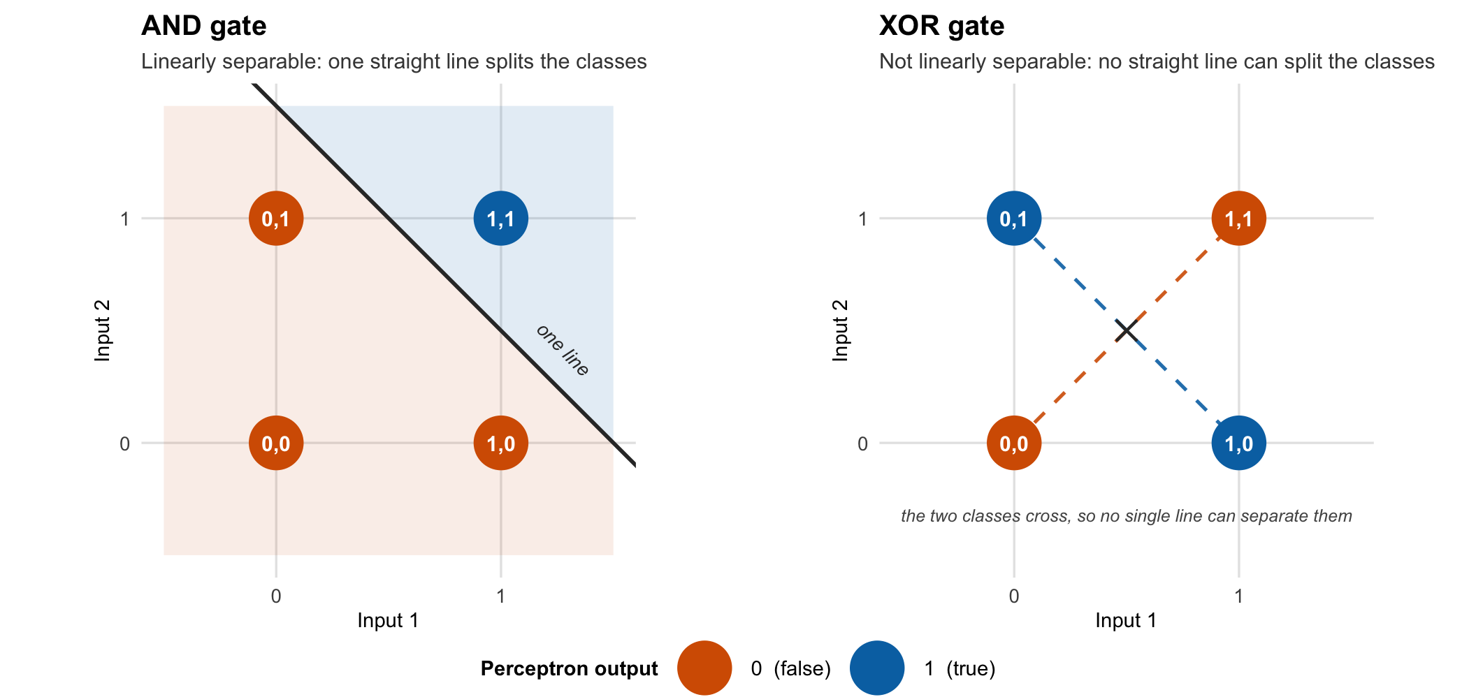
The XOR problem visualized: (Left) AND gate is linearly separable - a single line can divide the red and blue points. (Right) XOR gate requires at least two lines to separate the classes, which a single-layer Perceptron cannot learn.

Why XOR Matters:

The Perceptron makes decisions by drawing a line (or hyperplane in higher dimensions). Everything on one side of the line is class A, everything on the other side is class B. This works for problems like AND: The function places three points ((0,0), (0,1), (1,0)) with output 0 on one side of any potential line, while (1,1) with output 1 sits on the other side.

But look at XOR. The points that should output 1 are (0,1) and (1,0) - diagonally opposite corners. The points that should output 0 are (0,0) and (1,1) - the other diagonal. No single straight line can separate these diagonals. You need at least two lines, creating regions. But a Perceptron can only create two regions, not four.

Minsky and Papert didn’t just show XOR was hard - they proved it was impossible for a single-layer Perceptron. Their proof was elegant and devastating.

Here’s the tragedy: Minsky and Papert knew multi-layer networks could solve XOR. They said so in their book. But there was a catch - nobody knew how to train them. If you had hidden layers between input and output, how did you know which hidden neurons to blame when the network made a mistake? They called it the credit assignment problem, and it seemed mathematically impossible.

So the field arrived at a strange impasse: the machine that could solve XOR clearly existed on paper, but the method to teach it did not. That single unanswered question - how to distribute blame across hidden layers - was enough to stall an entire research program, and the years that followed would show just how completely.

Part II: The AI Winter and the Rule Writers (1970-1985)

Where we areFunding collapse. Government reports turn hostile, research money disappears, and intelligence gets redefined as rules a person types in by hand. Those rules sell for a decade and then meet their own limit.

The collapse was swift and total. In 1969, neural networks were the future. By 1970, they were the past. It was as if someone had turned off the lights at a party - one moment there was music and laughter, the next, empty silence.

The immediate impact of Minsky and Papert’s book was devastating for neural network research. Graduate students abandoned their theses. Funding agencies redirected their grants. Conferences that had been standing-room-only became ghost towns. But to understand the AI Winter - a term coined by analogy to nuclear winter, suggesting a deep freeze that kills everything - we need to understand that it wasn’t just about neural networks failing. It was about the entire field of AI confronting the chasm between its promises and reality. We had promised thinking machines by 1970. What we had were toys that could barely recognize handwritten digits.

The Funding Crisis

The timing couldn’t have been worse. The late 1960s saw the U.S. deeply mired in Vietnam, hemorrhaging $25 billion a year (about $200 billion in today’s dollars) into a war that was going nowhere. Congress was scrutinizing every research dollar with the intensity of an audit. Senator Mike Mansfield, concerned about wasteful defense spending, had just passed his famous amendment requiring all DARPA-funded research to have a direct, demonstrable relationship to a military function. Basic research without a clear defense application no longer qualified.

Perceptrons that might someday read handwritten digits didn’t qualify. Neither did robots that could stack blocks, or programs that could prove theorems. DARPA’s budget for AI research dropped from $3 million in 1969 to almost nothing by 1974. The money didn’t just decrease - it vanished, like water in the desert.

In Britain, the situation was equally grim, if more politely executed. Sir James Lighthill, a renowned mathematician who had worked on supersonic flight and fluid dynamics, was commissioned by the Science Research Council to evaluate AI research. His 1973 report was not just critical - it was a calculated assassination.

Lighthill sorted AI into three categories. Category A encompassed automation and engineering - useful applications but essentially clever programming rather than true AI. Category B represented the core promise of AI: building genuinely intelligent, thinking machines. Category C covered studies of the central nervous system - legitimate neuroscience research but distinct from artificial intelligence.

His conclusion was stark: Category B had failed to achieve its goals and faced fundamental limitations. He introduced the concept of the “combinatorial explosion” - the exponential growth of possibilities in real-world problems. A chess program might evaluate 10 moves ahead in a toy problem, but real chess required evaluating 10^120 possible games. A blocks world program could stack five blocks, but a real robot in a real warehouse would face infinite variations of lighting, positioning, and physics. The gap between toy demonstrations and useful applications wasn’t just large - it was mathematically unbridgeable.

The BBC organized a televised debate between Lighthill and AI researchers. It was one-sided. Lighthill, urbane and confident, dominated the exchange. The AI researchers, used to friendly academic conferences, were unprepared for this kind of hostile scrutiny. Within months, his report ended virtually all government AI funding in Britain. Entire research groups were disbanded. Edinburgh University, which had one of the world’s leading AI labs, saw its funding cut to zero.

The result was a brain drain. Researchers fled to industry or rebranded their work. “Artificial Intelligence” became “Knowledge Engineering” or “Expert Systems” or “Decision Support Systems.” The phrase itself was toxic.

The Rise of Symbolic AI: Intelligence as Rules

With neural networks discredited and buried, AI researchers embraced a different paradigm entirely. Intelligence, they now declared, wasn’t about learning - it was about reasoning. The human mind wasn’t a network of neurons but a symbol processor, like a computer running software. We didn’t need to simulate biology; we needed to encode logic.

This approach, later dubbed “Good Old-Fashioned AI” (GOFAI) with a mixture of nostalgia and derision, had strong philosophical roots reaching back millennia. It aligned with the rationalist tradition from Aristotle through Leibniz - the dream that all reasoning could be reduced to calculation. Leibniz had imagined a universal language where philosophical arguments could be settled by computation: “Let us calculate!” he said. Now, three centuries later, AI researchers believed they could finally build his dream.

GOFAI also had practical advantages that made it irresistible to computer scientists: you could understand exactly what the system was doing and why. Every decision could be traced, every rule examined. When it failed, you knew why. When it succeeded, you could explain how. This transparency was comforting after the black-box mystery of neural networks.

Expert Systems: The Brief Golden Age

The breakthrough came with expert systems - programs that encoded human expertise as if-then rules. The idea was seductive in its simplicity: if human expertise was just accumulated knowledge, then we could bottle it like wine. Interview the experts, extract their knowledge as rules, implement those rules in code. It was industrial-age thinking applied to intelligence: mass production of expertise.

The promise was intoxicating. Imagine: the world’s best doctor available in every rural clinic. The greatest chemist working in every lab. The top financial advisor accessible to every investor. Democracy of expertise through technology. Companies saw dollar signs. Governments saw strategic advantage. The gold rush was on.

MYCIN (1976) was the poster child. Developed at Stanford by Edward Shortliffe, it diagnosed blood infections and recommended antibiotics. Its knowledge base contained about 600 rules like:

IF: The gram stain of the organism is positive
AND: The morphology of the organism is coccus  
AND: The growth pattern is chains
THEN: There is suggestive evidence (0.7) that the organism is streptococcus

Each rule had a certainty factor, allowing MYCIN to reason with uncertainty. In a formal evaluation, a panel of specialists rated MYCIN’s therapy recommendations acceptable about as often as those of infectious disease faculty - on its narrow slice of medicine, the program performed at the level of the experts. It seemed like a triumph.

DENDRAL (1969) was even earlier, developed by Edward Feigenbaum (the “father of expert systems”). It determined molecular structures from mass spectrometry data. Unlike MYCIN’s diagnostic reasoning, DENDRAL used a generate-and-test approach: propose candidate structures, predict their spectra, compare with observed data. It was so successful that chemists actually used it for novel structure determination.

By the early 1980s, expert systems were a billion-dollar industry. Companies like DEC saved millions using XCON to configure computer systems. American Express used an expert system for credit approval. Japan launched its Fifth Generation Computer Systems project, betting their technological future on logic programming and expert systems.

The Knowledge Acquisition Bottleneck

But cracks were showing. Building expert systems required “knowledge engineers” to interview domain experts and encode their expertise. This process was excruciating:

Knowledge acquisition proved far more difficult than anticipated. Experts often couldn’t articulate their decision-making process, defaulting to “I just know” when pressed for specific rules. Different experts provided conflicting rules for the same scenarios. Rules interacted in unexpected ways, creating logical contradictions. Edge cases multiplied exponentially as systems grew. Maintenance became increasingly difficult - adding one rule could break ten existing ones.

In medicine, we encountered this constantly. A cardiologist might say, “If the patient has chest pain and shortness of breath, consider myocardial infarction.” But what kind of chest pain? How severe? What about atypical presentations in women or diabetics? The expert “just knew” from experience, but couldn’t fully articulate the nuanced pattern recognition they performed.

The Brittleness Problem

Expert systems were brilliant within their narrow domains but catastrophically brittle outside them. MYCIN could diagnose bacteremia but was useless for viral infections. Show it a fungal infection, and it would confidently recommend antibiotics that wouldn’t work. It had no concept of “I don’t know.”

This brittleness wasn’t a bug - it was fundamental. The systems had no real understanding, just rules. They couldn’t reason by analogy, couldn’t learn from experience, couldn’t handle novel situations. They were like medical students who had memorized a textbook but had never seen a patient.

The Common Sense Problem: The most ambitious attempt to save symbolic AI came from Marvin Minsky himself. If the problem was that AI lacked common sense, then the solution was obvious: give it common sense. How hard could it be?

Very hard, it turned out. Minsky’s “frames” tried to capture stereotypical situations as structured templates with slots and default values. Roger Schank and Robert Abelson created “scripts” for event sequences - what happens when you enter a restaurant (host seats you, waiter brings menu, you order, food arrives, you eat, you pay). Douglas Lenat launched Cyc (from “encyclopedia”), aiming to encode all human common sense knowledge. By 1985, they had encoded thousands of facts: water is wet, things fall down, dead people stay dead, you can’t be in two places at once, rain makes things wet, fire is hot, glasses break when dropped.

But common sense was an ocean, and they were trying to capture it with a thimble. A four-year-old knows that if you turn a cup of water upside down, the water falls out - unless the cup has a lid, or it’s frozen, or you’re in space, or it’s actually a magic trick cup. Every rule had exceptions, every exception had exceptions. The knowledge engineers went mad trying to encode the obvious. One famously quit after spending six months trying to formally define “edge” (as in the edge of a table). The project continues to this day, now with over 10 million assertions. It still can’t match a toddler’s understanding of the world.

By the mid-1980s, symbolic AI was hitting the same wall the Lighthill Report had identified a decade earlier: systems that worked on toy problems collapsed on real-world complexity.

The Underground

While the mainstream chased rules and logic, the neural network believers went underground. They couldn’t get funding, couldn’t publish in top journals, couldn’t use the words “neural network” without ridicule.

But they had each other. David Rumelhart and James McClelland started the Parallel Distributed Processing group in San Diego. Geoffrey Hinton, exiled to Carnegie Mellon, kept pushing. They met in small workshops, circulated manuscripts by hand, and slowly, carefully, worked on the credit assignment problem.

They knew something the symbol manipulators didn’t: intelligence wasn’t about rules. It was about connection patterns. The brain didn’t run logical inferences; it settled into states. Memory wasn’t retrieval; it was reconstruction. Learning wasn’t programming; it was weight adjustment.

By 1985, the expert systems bubble was bursting. They cost too much, broke too easily, and couldn’t learn.

Part III: Backpropagation and the Return of Neural Networks (1986-1998)

Where we areA working training rule. Errors propagate backward through stacked layers, and networks learn to read handwriting and hold a sequence in mind. The first commercial use reads bank checks, though the networks stay shallow.

The solution to the credit assignment problem was hiding in every calculus textbook, waiting patiently like a key under a doormat that everyone had walked past for seventeen years.

In 1986, the San Diego PDP (Parallel Distributed Processing) group published their two-volume manifesto. It ran to some 1,200 pages. Buried in chapter 8 of volume 1 was a 40-page paper by David Rumelhart, Geoffrey Hinton, and Ronald Williams that would revive neural networks. They called their method “backpropagation.”

The idea itself was simple. When the network makes an error at the output, you use the chain rule from first-year calculus to figure out how much each weight contributed to that error. Then you adjust each weight proportionally. Work backward from output to input, layer by layer, propagating the error signal like a wave traveling upstream. Hence, backpropagation.

The tragedy - or perhaps the comedy - was that it wasn’t even new. Paul Werbos had described the exact same algorithm in his 1974 PhD thesis, titled “Beyond Regression.” But Werbos was an economist at Harvard studying social systems, not a computer scientist. His thesis was filed away in the economics library where no AI researcher would ever look. Seppo Linnainmaa had invented automatic differentiation in Finland in 1970, published in his master’s thesis in Finnish. Even earlier, Arthur Bryson and Yu-Chi Ho had described it for control theory in 1969. The solution had been rediscovered at least four times, unknown to each discoverer. The neural network community had spent seventeen years in exile for want of an algorithm that multiple people had already invented.

Backpropagation

How a neural network actually works

Before the chain-rule bookkeeping below fully clicks, it helps to have the picture underneath it: what one neuron does, why stacking them buys you anything, and what learning actually looks like as the weights settle. This is the one I would start with (3Blue1Brown builds a network up from a single neuron), and each of the others draws the same idea from a different angle, so if one framing does not land the next usually does. The last two let you literally watch a network train.

Backpropagation worked not because it was complex, but because it was simple enough to actually implement. The beauty was in its recursive elegance: the error at any layer could be computed from the error at the next layer. It was like a cascade of responsibility, each layer passing blame backward until every weight knew exactly how much it had screwed up.

The math was clean:

∂E/∂w_ij = ∂E/∂o_j × ∂o_j/∂net_j × ∂net_j/∂w_ij

That is the chain rule, and each of its three terms is a plain question. How wrong was the output? How sensitive was this neuron to its own incoming signal, meaning does nudging its input move its output at all? And how much did this particular weight actually contribute, which is just the value that flowed along it.

Take the smallest network that has a hidden layer: one input, one hidden neuron, one output. The input is 1.0. The weight into the hidden neuron is 0.5, so the hidden neuron receives 0.5 and, after squashing, emits 0.6; its activation curve has slope 0.5 at that point. The weight from hidden to output is 2.0, so the output neuron receives 1.2 and emits 0.8, with slope 0.25 there. We wanted 0.5, so we are off by 0.3.

Now walk it backward. At the output, multiply the error by the output neuron’s own sensitivity: 0.3 × 0.25 = 0.075. Call that the output’s blame. The gradient for the second weight is that blame times what flowed along it: 0.075 × 0.6 = 0.045.

Then push the same 0.075 one layer up. Send it through the weight it came in on and through the hidden neuron’s sensitivity: 0.075 × 2.0 × 0.5 = 0.075 is the hidden neuron’s blame, and its weight’s gradient is 0.075 × 1.0 = 0.075.

Notice what happened. The 0.075 computed at the output was not recomputed for the hidden layer; it was handed up and reused. That reuse is the whole algorithm. One backward sweep prices every weight in the network, because each layer inherits the layer below’s answer instead of deriving it from scratch. Do it in the other direction and you would have to trace a separate path from each individual weight all the way forward to the output, once per weight, which for a network of any size is hopeless. Backward, the cost is roughly one extra pass. Forward, it scales with the number of weights.

3Blue1Brown’s chapter 3 is the same backward pass done visually, if you would rather watch the blame spread than read it.

And if you learn by building: Karpathy codes backprop from scratch here. It’s the moment the whole thing stops being abstract.

They demonstrated it on XOR - the problem that had killed the field. The network learned it easily. They tried harder problems. The network learned those too. Neural networks were back.

The Art of Teaching Networks

Backpropagation told you which direction to adjust weights. But how much? Too little and training took forever. Too much and you’d overshoot, oscillating wildly. This was the art of optimization - navigating mountainous loss landscapes in thousands of dimensions.

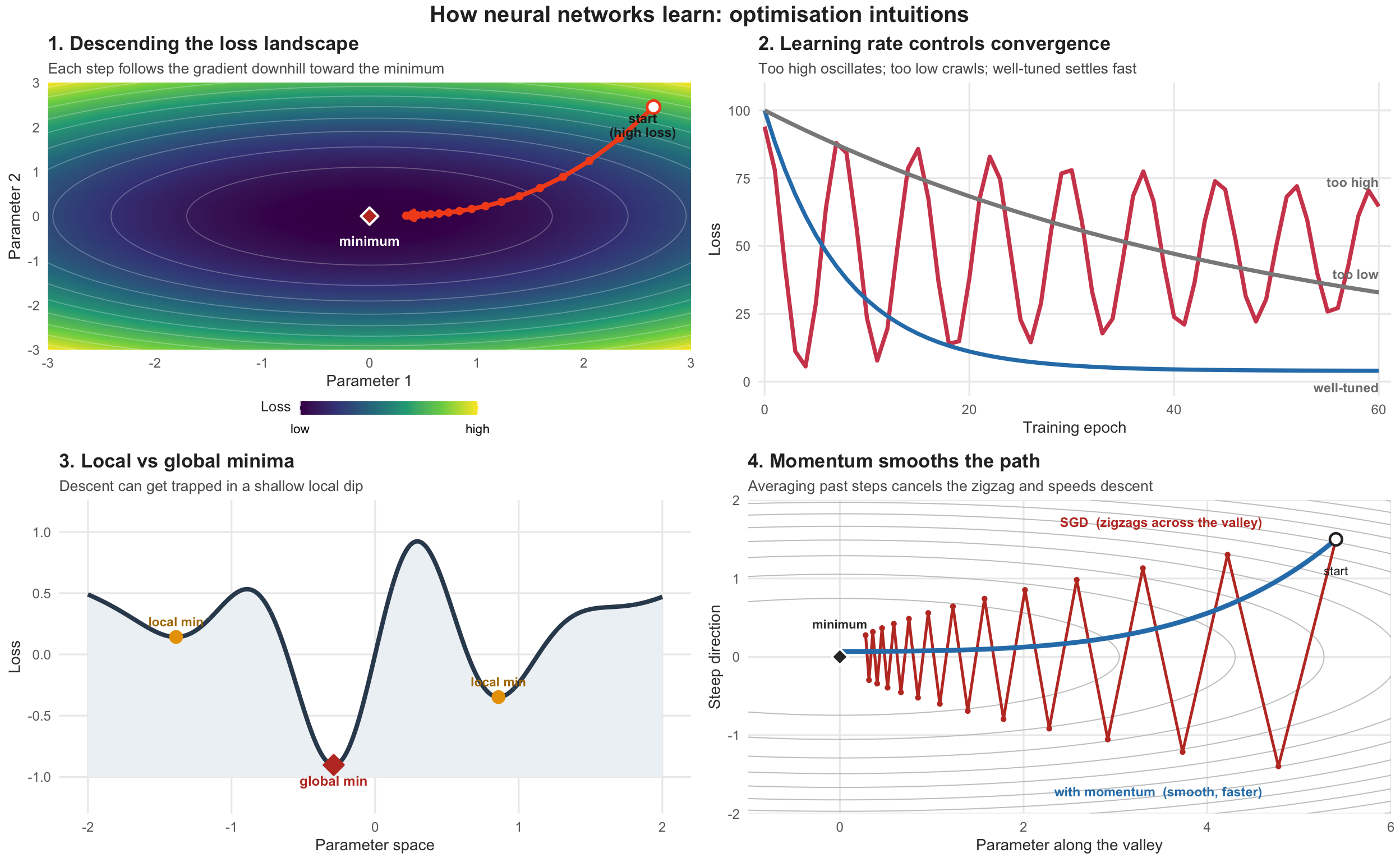
Those four panels are worth sitting with, because between them they cover most of what training a network actually feels like. Panel 1 shows a tidy bowl; a real loss surface has millions of dimensions and all you ever see is the slope under your own feet. Panel 2 is the parameter I have spent the most time fiddling with: too large a step and you bounce across the valley instead of down it, too small and you are still descending when the funding runs out. Panel 3 shows the trap everyone feared for years, and it turned out to matter less than expected, because wide networks have so many directions available that most of the dips you land in are about as good as one another. Panel 4 is the fix for the zigzag: average your recent steps, the side-to-side cancels itself out, and the one direction you keep agreeing on survives.

Convolutional Neural Networks: Building in a Priori Knowledge (1989)

How machines learned to see

A convolution is one of those operations that only clicks once you watch a kernel slide across an image. These are the clips that made it click for me, in the order the idea actually built up: the operation itself, then the architecture that stacks convolutions into a vision system, then a look inside at what the layers have actually learned. Watch them in sequence and the diagrams below stop being boxes and arrows.

Before the architecture makes sense, it helps to see exactly how badly the networks of the previous section handle an image. Take a 28×28 grayscale digit. To feed it into a fully connected network you first have to unroll it into a list of 784 numbers, then wire that list into the first hidden layer. If that layer has 1000 units, every one of the 784 inputs connects to every one of the 1000 units: about 800,000 weights in the first layer alone, before the network has detected anything at all. Every one of those weights has to be learned from data.

The parameter count is the smaller problem. The real problem is that unrolling destroys the fact that the numbers came from a grid. Nothing in the input vector says that pixel 100 sits directly beside pixel 101, or above pixel 128. So take a handwritten 3, shift it two pixels to the right, and you hand the network a substantially different vector: different values in different slots, with no hint that it is the same digit. Whatever the network learned about threes in the middle of the frame buys it nothing on the right side of the frame. It has to learn the digit again at every position it might appear, from training examples that happen to show it at every position. It is a bit like training a resident to spot mitotic figures only in the upper left of the field, then starting the training over for the upper right.

The fix is to stop pretending the image is a bag of numbers and build the geometry into the architecture itself: let each unit look at a small local patch, and let the same detector be reused everywhere on the image rather than relearned. The figure below is what that looks like when you stack it into a full network, and the one after it zooms in on the single operation doing the work.

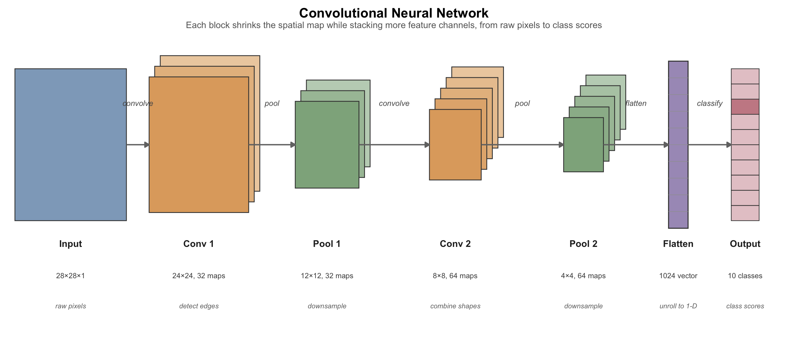
CNN layers work together: Convolution detects patterns (edges→shapes→objects), Pooling reduces size while preserving important features, Fully Connected combines all features for final classification.

The trade running left to right in that diagram is worth naming: the spatial map keeps shrinking, from 28×28 down to 4×4, while the number of feature channels keeps growing, from one grayscale image to 64 maps. The network is gradually giving up precise location and buying, in exchange, a larger vocabulary of things it can recognize. Only at the very end, once the map is small and the vocabulary is rich, does it flatten everything into a vector and hand it to an ordinary fully connected classifier. The next figure shows one convolution in isolation.

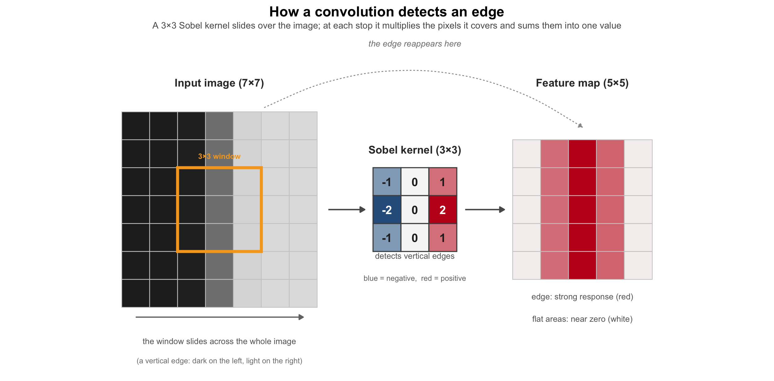
The convolution operation: A small kernel slides across the image, computing dot products to detect specific patterns like edges.

It is worth reading that figure slowly, left to right. The 7×7 grid on the left is the input. Its first three columns are nearly black, its last three are nearly white, and the single column between them is mid-gray. That dark-to-light column is the whole content of the image: a vertical edge, the kind of boundary you see wherever a dark structure meets a lighter background.

The 3×3 grid in the middle is the kernel, in this case a Sobel vertical-edge detector. Its left column holds negative weights, its middle column zeros, its right column positive weights, which is why it renders blue on the left and red on the right. The operation is simple arithmetic: drop the kernel over any 3×3 patch of the image, multiply each of the nine weights by the pixel sitting underneath it, and add up the nine products. That gives you one number. Then move the window one pixel over and do it again.

The number comes out strongly positive when the patch is dark on the left and light on the right, because the negative weights land on small values and the positive weights land on large ones. It comes out near zero over a uniform patch, dark or light, because the negative and positive contributions cancel each other out. Slide the window over every valid position in a 7×7 image and you collect 25 such numbers, which is the 5×5 feature map on the right. Look at where the color is: the loud red stripe runs down its middle column, exactly the stops where the window straddled the boundary. The flat regions on either side come out near white. Nobody told the kernel where the edge was. It found the edge by being run everywhere and reporting where it fired.

That last point is the whole idea. Nine numbers were enough to check the entire image for vertical edges, and the same nine numbers worked at every position. This is what LeCun turned into an architecture.

Yann LeCun’s Insight: Weight Sharing (1989)

While everyone else was building fully connected networks - where every neuron talked to every other neuron - Yann LeCun was drawing on what Hubel and Wiesel had discovered in cat visual cortex decades earlier.

Hubel and Wiesel had won the Nobel Prize for discovering that visual neurons were arranged in a hierarchy. Early neurons detected edges. Later neurons combined edges into shapes. Even later neurons recognized objects. And crucially, each neuron only looked at a small patch of the visual field.

LeCun realized this wasn’t an accident - it was an engineering solution. Images have local structure. Pixels near each other are related. Patterns repeat across the image. Why make the network learn what evolution had already discovered?

His Convolutional Neural Networks built these insights directly into the architecture, as three constraints that each answer one of the failures above.

Local connections came first. Each neuron looked only at a small window, something like 5×5 pixels, rather than at all 784 inputs. Since the things that make an edge an edge are all within a few pixels of each other, the long-range connections were mostly wasted capacity anyway. Dropping them cut the parameter count by roughly 99%.

Weight sharing was the sharper move. Rather than learn a separate detector for each location, the same small set of weights - one kernel, exactly like the Sobel kernel above - slid across the entire image. If the network learned to spot a vertical edge in the upper left, it could spot that edge anywhere, for free, because it is literally the same nine numbers being applied everywhere. The shifted-digit problem largely dissolves: the detector moves with the feature.

Pooling handled what was left. After a bank of detectors has run, you shrink the feature map by summarizing each small neighborhood with a single number, usually the largest value in it. You lose the feature’s exact address and keep the fact that it was present nearby. What that buys is tolerance to small shifts: an edge that lands at pixel 12 in one image and at pixel 14 in the next falls into the same pooling neighborhood and produces the same output, so the layers downstream cannot tell the two apart and do not need to. Stack a few pooling steps and the network stops caring about a few pixels of jitter in handwriting, in framing, or in where a slide sits under the objective.

Put together, the three constraints reproduce the hierarchy Hubel and Wiesel had mapped: small receptive fields early, progressively larger and more selective ones deeper in, with position sensitivity traded away layer by layer for abstraction. That correspondence is real, and it is also the design you converge on from the engineering argument alone, which is part of why it is convincing. But it is worth being honest about the direction of the borrowing. LeCun has consistently described the visual cortex as inspiration rather than a specification: he was not transcribing a circuit diagram, cortical neurons do not share weights in the literal sense the algorithm does, and nothing in the brain is known to run backpropagation. Biology suggested where to look. The reason the architecture held up is that the constraints turned out to be true things about images.

By 1998, LeCun’s LeNet-5 was reading millions of handwritten checks for banks - by some accounts a noticeable fraction of all checks processed in the United States. Neural networks weren’t just back - they were making money.

The Memory Problem (1990-1997)

Images were spatial. Language was temporal. You couldn’t understand “bank” without knowing if the previous words were “river” or “financial.” Networks needed memory.

Jeffrey Elman’s answer was elegant: connect the network to itself. Take the hidden layer’s activation and feed it back as input on the next time step. Now the network had memory - it could remember what it had seen.

Except it couldn’t. Not really. The memory faded exponentially. After 5-7 words, the network had forgotten everything. They called it the vanishing gradient problem. It was diagnosed properly in 1991 by a graduate student in Munich named Sepp Hochreiter, in a thesis almost nobody read at the time - remember his name, because the person who diagnosed the disease also built the cure. As you backpropagated through time, the gradient got multiplied by weights at each step. Small weights? The gradient vanished to zero. Large weights? It exploded to infinity.

A clear walkthrough of why plain RNNs forget, and how the LSTM’s gates let information survive across long sequences.

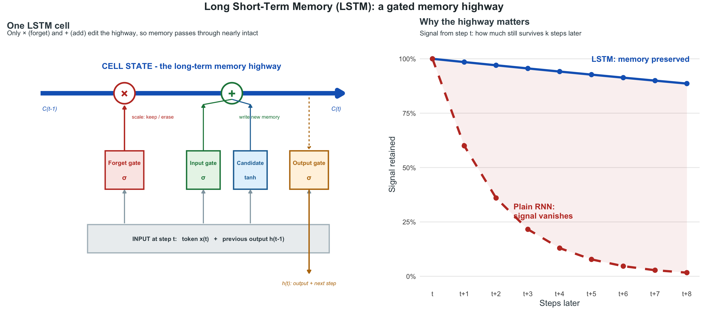
LSTM architecture: Three gates (forget, input, output) control information flow, allowing networks to remember important information for hundreds of time steps.

Long Short-Term Memory (1997)

Sepp Hochreiter - the same student who had diagnosed the vanishing gradient six years earlier - was Jürgen Schmidhuber’s PhD student in Munich. His thesis was radical: don’t fight the vanishing gradient, engineer around it.

The Long Short-Term Memory (LSTM) network was like a computer memory cell built from neurons. It had gates - neural circuits that decided what to remember, what to forget, and what to output. The key innovation was the “cell state” - a highway that let information flow unchanged across time.

Here is why that defeats the vanishing gradient. In a plain recurrent network, the signal is re-multiplied by the weights at every single step, so a hundred steps means a hundred multiplications and anything below one collapses toward zero. The cell state is different: it is added to, and touched by only a single gate, so a memory can ride along it for hundreds of steps without being multiplied away. Change the operation from repeated multiplication to addition, and the gradient survives the trip.

It was complicated. The original had two gates, input and output; the now-familiar forget gate was added later, by Gers and colleagues in 2000. Critics called it baroque. But it worked. LSTMs could remember for hundreds of time steps. They could learn when to store information, when to access it, when to forget it.

For the next twenty years, until transformers arrived, LSTMs were how we did language AI. Google Translate, Siri, Alexa - all ran on LSTMs.

That success story runs ahead of us, though. While neural networks were slowly reclaiming language, a different family of methods owned the 2000s - and to see why, we need to rewind to 1999.

Part IV: Statistics and Hand-Built Features (1999-2012)

Where we areA statistician's decade. Kernels, ensembles, and probability win the benchmarks while hand-written rules fade out. Every winning method shares one requirement: a person decides in advance what the machine should look at.

The probability underneath

This whole era ran on statistics, so before the SVMs and boosted trees below start quietly assuming you know why a Gaussian turns up everywhere or how a prior reshapes a diagnosis, these are the clearest intuitions I have found for that substrate. I paired 3Blue1Brown's geometry with Josh Starmer's step-by-step walkthroughs on purpose: one gives you the why, the other the how. Bayes and the medical-test paradox are the two I send to every resident.

The late 1990s exposed an uncomfortable reality: neural networks, despite their biological inspiration and recent revival, were being systematically outperformed by methods with stronger theoretical foundations.

At KDD Cup 1999, the premier data mining competition, the top 10 submissions all used decision trees or rule-based systems. In bioinformatics, SVMs routinely outperformed neural networks on tasks like protein classification. The pattern repeated across domains: document classification, credit scoring, medical diagnosis. Neural networks had become a cautionary tale about the gap between biological metaphor and practical engineering.

The fundamental issue wasn’t theoretical - it was infrastructural. Neural networks demanded three preconditions that simply didn’t exist: 1. Data abundance: Networks needed millions of examples; we had thousands 2. Computational density: Backpropagation required matrix operations that CPUs handled poorly 3. Architectural knowledge: The space of possible architectures was vast and we were navigating blind

Until this trinity aligned, statistical methods offered a superior value proposition: theoretical guarantees, computational efficiency, and interpretable decisions.

Statistical Learning and Ensemble Methods

Kernels, trees, and ensembles

Before deep learning took over, these were the methods that actually won the bake-offs, and nobody makes them click like Josh Starmer. StatQuest is the friendliest visual take on the max-margin idea and the kernel trick, and the run continues through trees, forests, and the boosting that still rules tabular data. Luis Serrano's SVM intro is the geometric companion I keep going back to. In order, they turn this era from a grab-bag of algorithms into one connected story.

During the late 90s and early 2000s, while deep learning was still struggling, more traditional statistical methods dominated.

Support Vector Machines: Maximum Margin Classification

Vladimir Vapnik’s SVMs (1995) approached classification with geometric elegance: find the hyperplane that maximizes the margin between classes. The idea is easier to hold onto if you stop thinking about hyperplanes for a moment and think about a street. You have two clouds of points, one class on each side, and you want to draw a boundary between them. There are infinitely many lines that separate the training data perfectly, and if all you care about is the data you already have, they are all equally good. But you do not care about the data you already have. You care about the next patient, the next transaction, the next sample. So the question becomes: which of those infinitely many lines is most likely to still be right tomorrow? Vapnik’s answer was the one that runs down the middle of the widest possible street between the two classes. If the boundary is crowded up against one class, a new point drawn from that same class only has to wobble slightly to land on the wrong side. Push the boundary to the center of the widest gap and every point gets the maximum amount of room to wobble before it is misclassified. Margin, in other words, is a way of buying tolerance for the noise you have not seen yet.

What falls out of that framing is a fact that surprised me the first time I understood it. Once you have found the widest street, the boundary depends only on the handful of points that touch its edges. Those are the support vectors. Every other point in the training set could be moved, or deleted outright, and the boundary would not shift by a millimeter, because those points are not what is holding the street to its width. Practically, this means the model is defined by a few dozen examples out of thousands, which makes it compact and fast to evaluate. Conceptually, it tells you where the information about the boundary actually lives: at the edges of each class, in the ambiguous cases, not in the comfortable middle. This is the same reason a pathologist learning to grade a tumor spends most of their time on the borderline cases. The unmistakable ones teach you very little about where the line is.

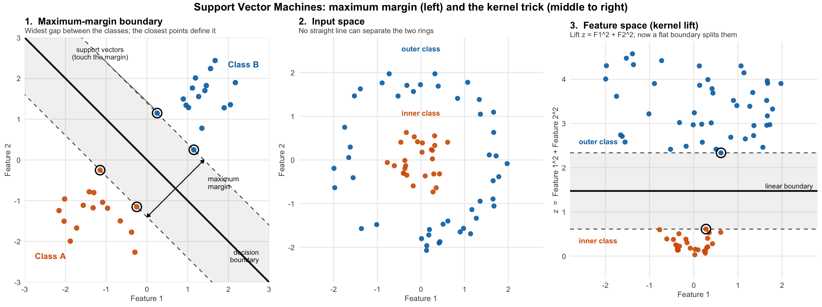
The problem, of course, is that most interesting data is not separable by a straight line at all. The middle panel above shows the standard example: one class in a central blob, the other in a ring around it. No line, anywhere, at any angle, splits those two. The classic escape is to add a dimension. If you compute a new feature z equal to the squared distance from the origin, the inner class sits low and the outer class sits high, and now a flat boundary in that lifted space separates them cleanly. Project the flat boundary back down and it becomes a circle in the original space. Curved decision boundaries are just straight boundaries viewed from a space with more dimensions in it.

The kernel trick is what makes that escape practical rather than merely cute. Lifting into a higher-dimensional space is expensive, and for some useful transformations the target space is infinite-dimensional, so you cannot compute the coordinates even in principle. The saving observation is that the SVM optimization never asks for a point’s coordinates. It only ever asks for dot products between pairs of points. So if you can find a function that returns the dot product two points would have had in the lifted space, computed directly from their original coordinates, you get the curved boundary without ever visiting the higher-dimensional space. That function is the kernel. The linear kernel, K(x,y) = x·y, is the no-op that gives you the plain straight boundary. The polynomial kernel, K(x,y) = (x·y + c)^d, corresponds to a space of all feature interactions up to degree d, which would be a large number of explicit coordinates and is instead one multiplication and one exponent. The RBF kernel, K(x,y) = exp(-γ||x-y||²), corresponds to an infinite-dimensional space and is still just a subtraction, a norm, and an exponential. You choose the shape of the boundary by choosing a similarity function, and the cost barely moves. That combination of a clear geometric objective, a compact model defined by a few support vectors, and boundaries of arbitrary curvature for almost no extra compute is why SVMs were the method to beat for most of a decade.

Decision Trees: Learning by Splitting (CART - 1984)

Before Random Forests, we need to understand CART (Classification and Regression Trees), developed by Leo Breiman and colleagues. CART is a fundamental example of supervised learning, in which the algorithm learns patterns from labeled training data to make predictions on new data. The learning procedure is close to how a clinician builds a triage rule, and it is worth stating plainly: start with all the data at the root, and ask which single yes-or-no question about a single variable does the most to sort the outcomes apart. To answer that, the algorithm tries every variable at every possible split point and scores each candidate. For classification, the score is a purity measure such as Gini impurity or entropy, which is low when a group is mostly one class. For regression, it is the variance within the resulting groups. Whichever question produces the cleanest two children wins. Then the same procedure runs again independently inside each child, and again inside their children, until a node is pure, or holds too few samples to split responsibly, or hits a preset depth limit.

A worked example makes the recursion concrete. Imagine predicting whether someone will default on a loan. The first split turns out to be income below $50K, because that question buys the largest reduction in variance. The left branch, the lower-income group, has an 80% default rate, and the right branch has 20%, so neither is pure and both are worth splitting further. Splitting the left branch again on credit score below 600 sends 95% default into one leaf, which is pure enough to stop, and 60% default into the other, which still has work to do. You continue in this fashion until every leaf is reasonably homogeneous, and what you are left with is a flowchart.

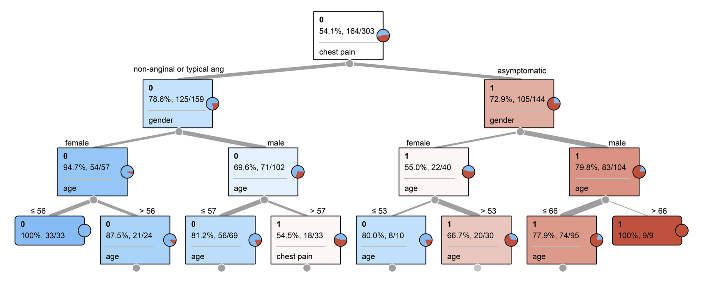Decision Tree Example A real CART decision tree: Each split maximizes information gain, creating a flowchart for predictions. New data follows the learned path to a prediction.

Prediction is then trivial, which is a large part of the appeal. A new instance starts at the root, answers each question with its own feature values, follows the corresponding branch, and lands in a leaf that reports either a class probability or a regression value. Nothing is normalized, nothing is scaled, and the whole path is inspectable, so you can say exactly why a given prediction came out the way it did. That transparency, plus the ability to capture non-linear structure through repeated splitting, is why trees survived every wave of fashion in this field.

The failure modes are just as characteristic. Left to grow unchecked, a tree will keep splitting until it has effectively memorized the training set, carving out leaves that describe individual quirks rather than real structure. Trees are also unstable: change a handful of training rows and the first split may change, and because everything below is conditional on that split, you can get a visibly different tree from nearly identical data. They are greedy, always taking the strongest predictor first without considering whether a weaker split now would open up a better one later. And because each split is a threshold on one variable, the boundaries are axis-aligned staircases, which is an awkward way to approximate a diagonal. Two of those weaknesses, instability and overfitting, turn out to be exactly what the next idea exploits.

Random Forests: The Wisdom of Trees

Leo Breiman’s insight (2001) was to stop fighting the instability and use it. If a single tree is high-variance, train many trees and let them vote, and the errors that are specific to each tree should cancel while the signal they share reinforces. The catch is that averaging only helps if the trees actually differ. Feed a hundred trees the same data with the same features available and they will all find the same first split, the same second split, and the same mistakes, and a hundred identical opinions are worth exactly one opinion. So the real work in Random Forests is manufacturing genuine disagreement, and Breiman did it along both axes of the data matrix.

The first mechanism is bagging, short for bootstrap aggregating: each tree is trained on its own random sample of the rows, drawn with replacement, so every tree sees a slightly different version of the training set and some examples appear twice while others are left out entirely. The second mechanism, and the one that does most of the work, is random feature selection: at each split, a tree is only allowed to consider a random subset of the columns, conventionally about the square root of the total number of features for classification. This is not a hint or a penalty. The tree literally cannot see the other variables at that moment, and has to build the best question it can out of what it was dealt.

Why that column restriction matters is easiest to see with a dominant predictor. Imagine you have 100 features, and “Income” always dominates. Under the traditional approach, every tree splits on Income first, and you end up with a hundred near-copies of the same tree. Under a Random Forest, Tree 1 might be dealt [Age, Education, ZIP, …] with no Income at all, Tree 2 gets [Income, Gender, Credit Score, …], and Tree 3 gets [Employment, Debt, Region, …] with no Income either. The result is that each tree must learn different patterns because they literally cannot access the same features. Tree 1 discovers what Age and Education can tell you, Tree 3 finds the Employment and Debt relationship, and the forest ends up holding several independent accounts of the same phenomenon instead of one account repeated a hundred times. Hiding the obvious variable from most of the trees is what forces the rest of the signal in the data to be discovered at all.

The arithmetic of the ensemble follows from that. Any individual tree, working from a partial view of the rows and a partial view of the columns, might be only 60 to 70% accurate on its own, which sounds like a poor model. But the trees are wrong in different places, because they were built from different information, so when a hundred of them vote the individual mistakes are outvoted and the shared signal survives. Combined accuracy in the 85 to 95% range from components that weak is the whole point: the collective sees the patterns that no single restricted view could. It is also why the forest gives up the one thing the single tree was best at. You can still ask which variables mattered on average, but you can no longer trace a prediction down one readable path, because the answer is a tally across a hundred of them.

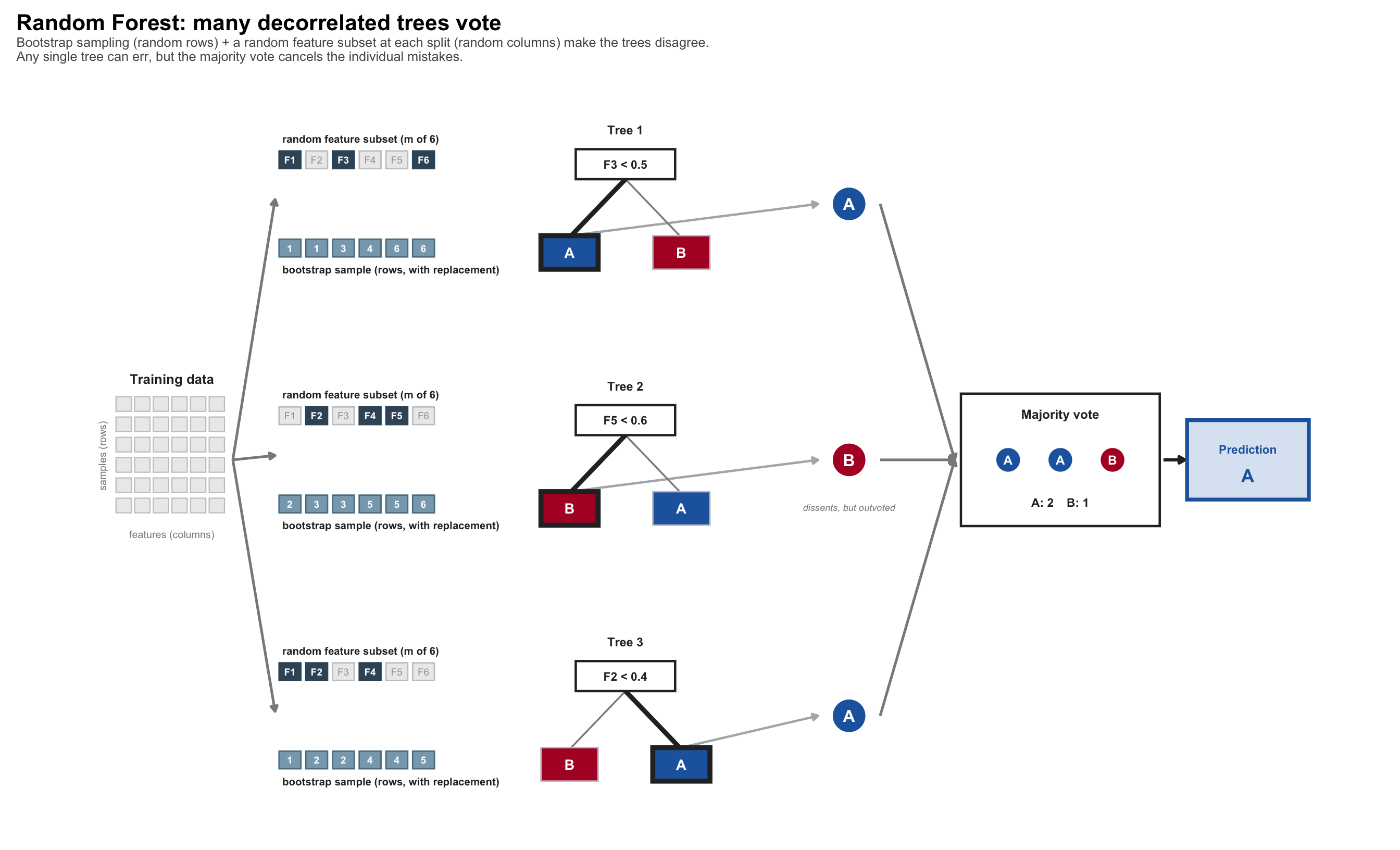
The Statistical Learning Toolkit

By 2010, machine learning had become a toolkit of specialized methods: - SVMs for maximum margin classification - Random Forests for anything with structured/tabular data
- Gradient Boosting for competition-winning accuracy - Logistic Regression when you needed interpretability - k-Nearest Neighbors for local patterns

Neural networks? They were the weird kid in the corner, theoretically powerful but practically useless. Too hard to train, too easy to overfit, too computationally expensive.

That was about to change.

For all its range, the statistical toolkit still shared one limit: every method leaned on a person deciding, in advance, which features mattered. By 2012 that approach was about as strong as hand-engineering would ever make it. The next leap came from a different idea, networks that learned their own representations of the world, discovering the structure we had been building by hand. That is the story of Part V.

Part V: Deep Learning and the ImageNet Result (2012-2016)

Where we areFeatures found, not built. Cheap parallel hardware, a million labeled photographs, and better training tricks arrive together, and hand-designed features stop mattering. The same approach then wins at speech and at Go.

September 30, 2012.

The ImageNet competition results were posted. A team from the University of Toronto - not Stanford, not MIT, not Google - had come in at a 15.3% error rate. The previous best was 26.2%, a gap of almost eleven percentage points and far larger than the field’s usual year-over-year gains.

Geoffrey Hinton, who had kept working on neural networks through years when most of the field had moved on, was behind it.

Three Things Converged (2006-2012)

For neural networks to compete with statistical methods, three separate things needed to align: large labeled datasets, fast parallel hardware, and a handful of training techniques. Between 2006 and 2012, they did.

Data Availability

The internet provided unprecedented amounts of labeled data. Suddenly we had billions of labeled images on Flickr, countless hours of transcribed speech on YouTube, and the entire web’s text to train on. Fei-Fei Li spent three years building ImageNet - 14 million images, hand-labeled using Amazon Mechanical Turk. It cost hundreds of thousands of dollars. It would prove to be worth billions.

Computational Hardware

In 2007, NVIDIA released CUDA, letting researchers program graphics cards for general computation. GPUs were built for video games - calculating millions of pixels in parallel. Turns out, neural networks are the same thing: millions of parallel matrix multiplications. A $500 gaming GPU could outperform a $10,000 CPU cluster. Andrew Ng proved it in 2009, training networks 70x faster on GPUs.

Algorithmic Improvements

Researchers discovered a collection of “tricks” that suddenly made deep networks trainable:

ReLU (2010): Everyone used sigmoid activations because they looked biological. But they had a fatal flaw: gradients vanished. The fix was embarrassingly simple: f(x) = max(0, x). Just return zero for negative inputs, x for positive. No saturation, no expensive exponentials. Networks trained 6x faster.

Dropout (2012): Geoff Hinton’s idea sounded reckless: randomly delete half your neurons during training. His student Nitish Srivastava implemented it, and it worked - forcing the network to be robust, no single neuron could dominate. Overfitting dropped by 50%.

Better Initialization (2010): Xavier Glorot realized weight initialization was critical. Too small: gradients vanish. Too large: gradients explode. Scale by 1/√n where n is the number of inputs. One line of code that made 10-layer networks suddenly trainable.

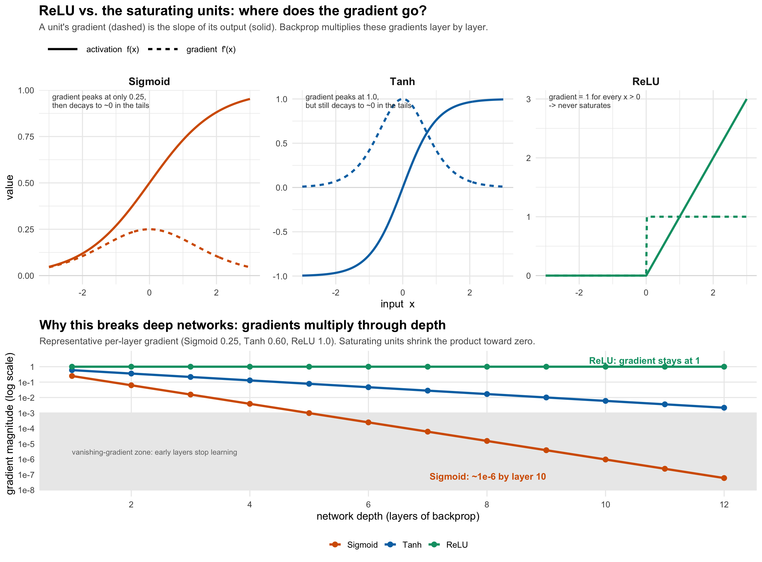
ReLU’s strength was its simplicity. While Sigmoid and Tanh suffer from vanishing gradients in deep networks, ReLU maintains constant gradient flow, enabling training of much deeper architectures.

Bigger networks and better training are only half of the Part V story. The same years produced a quieter shift: some models were beginning to learn what their data meant on their own, with no labels at all. The clearest early example came from language.

AlexNet and the ImageNet Competition (2012)

My favorite video on this whole page. Welch Labs actually shows you what AlexNet learned inside, edges then textures then object parts, which is the part the text can only describe.

On September 30, 2012, the ImageNet Large Scale Visual Recognition Challenge results were announced. Geoffrey Hinton’s team from the University of Toronto - Alex Krizhevsky, Ilya Sutskever, and Hinton himself - submitted a convolutional neural network they called AlexNet.

The previous state-of-the-art methods relied on hand-crafted features like SIFT (Scale-Invariant Feature Transform), HOG (Histogram of Oriented Gradients), and Fisher Vectors. These approaches had plateaued around 26% error rate for two years. AlexNet achieved 15.3% error - a relative improvement of 41% over the 26.2% second-place result.

AlexNet’s architecture consisted of five convolutional layers followed by three fully connected layers, totaling 60 million parameters. The network was trained on 1.2 million ImageNet images using two GTX 580 GPUs over the course of a week - a task that would have taken approximately three weeks on contemporary CPUs.

Several technical choices contributed to AlexNet’s success. ReLU activations enabled faster training and better gradient flow compared to traditional sigmoid or tanh functions. Dropout with probability 0.5 in the fully connected layers reduced overfitting. Data augmentation - extracting random 224×224 patches from 256×256 images, applying horizontal flips, and adding color jittering - effectively increased the training set size. The use of GPUs provided the computational power necessary for training such a large network.

This result marked a fundamental shift in computer vision. Within a year, nearly all competitive entries to computer vision challenges used deep convolutional networks. The era of manual feature engineering in vision had ended.

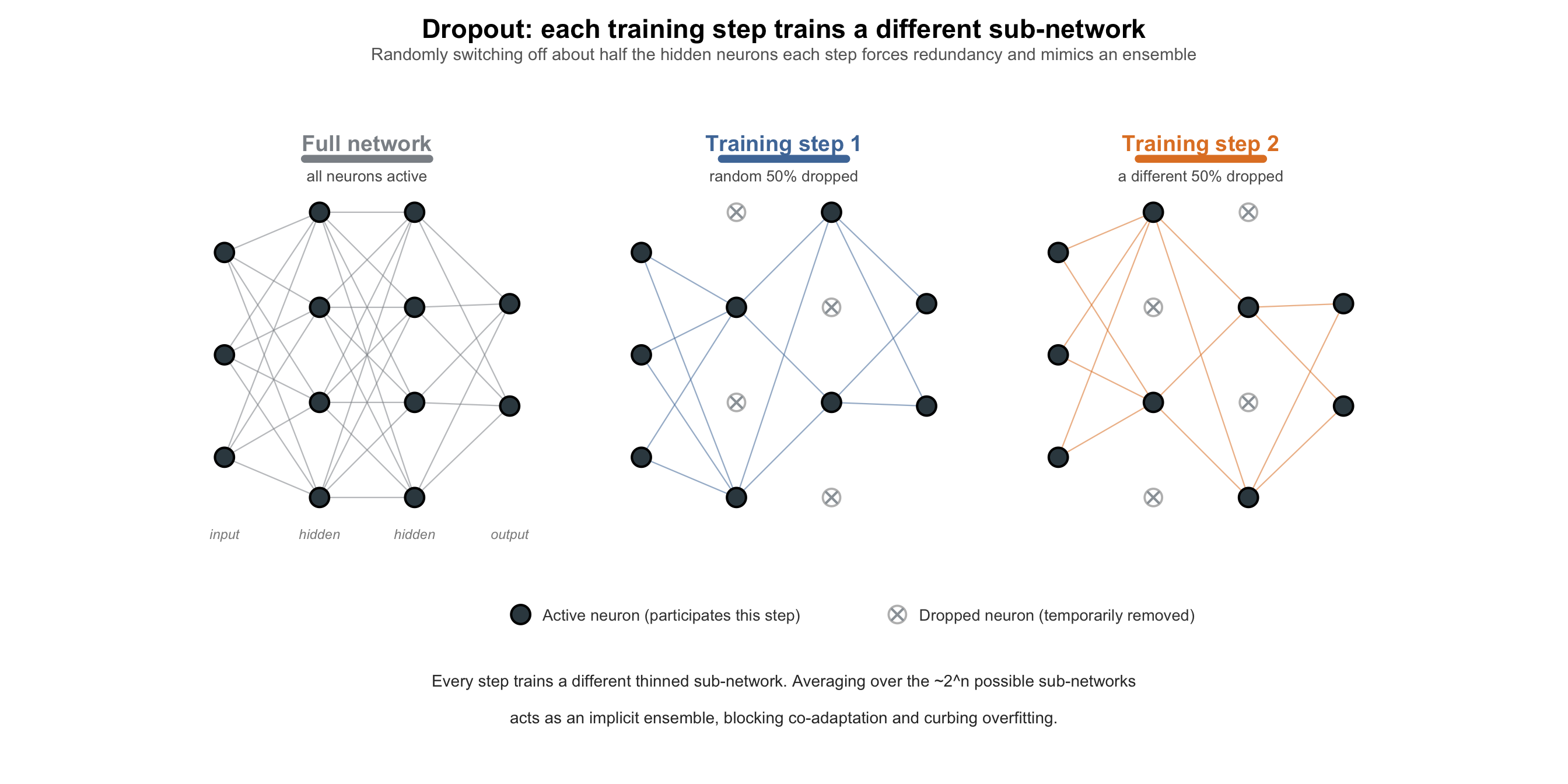
Dropout forces the network to be robust by randomly removing neurons during training. No single neuron can dominate - the network must learn redundant representations.

Word Embeddings: Self-Supervised Learning Discovers Meaning (2013)

The linear algebra of meaning

Everything from here on treats meaning as geometry: words become vectors, similarity becomes an angle, and attention is ultimately just a lot of dot products. If that sentence felt like hand-waving, this shelf is the fix. Grant's Essence of Linear Algebra is the best math series on the internet, and the dot-product chapter in particular is the single operation attention runs on. PCA and SVD at the end are how you actually look at these high-dimensional spaces.

Rob Miles gives a genuinely honest tour of word vectors here, including where the king − man + woman analogy holds up and where it quietly breaks.

A crucial missing piece for language understanding was a better way to represent words. In 2013, Tomas Mikolov at Google created Word2Vec, demonstrating the power of self-supervised learning - the model learned meaningful representations without any labeled data, just raw text.

The breakthrough: Word2Vec predicted context words from a target word (Skip-gram) or vice versa (CBOW). This simple task - predicting nearby words - forced the model to learn that words appearing in similar contexts must have similar meanings. No human told it that “cat” and “dog” were related; it discovered this by observing they appear near words like “pet,” “furry,” and “walked.”

Through this self-supervised objective, Word2Vec learned dense vector representations where semantic relationships were captured geometrically. The famous example: vector('king') - vector('man') + vector('woman') resulted in a vector very close to vector('queen'). The model discovered that gender, royalty, geography, and countless other relationships could be encoded as consistent directions in vector space.

The Power of Self-Supervised Learning:

Word2Vec proved that you don’t need labeled data to learn meaning - just observe how words are used. By predicting context, the model discovered that many semantic relationships show up as directions in space. The offset that carries “man” to “king” roughly carries “woman” to “queen”, and the offset that carries “Paris” to “France” roughly carries “Tokyo” to “Japan”. No one labeled those relationships; they emerged from the single objective of predicting nearby words.

The same objective organized the space by usage. Words that appear in similar contexts ended up near each other - medical terms in one region, colors in another, emotions in a third. That structure was never programmed; it fell out of training.

It is worth being honest about the limits. These analogies are approximate and somewhat cherry-picked. The famous king − man + woman ≈ queen result holds for a handful of well-chosen examples, and the arithmetic is far messier for most words. The structure is real, but it is not a precise algebra of meaning.

This principle - that models could learn rich representations from the structure of data rather than from explicit labels - became foundational to modern NLP. BERT (2018) extended it with masked language modeling, predicting randomly hidden words from context. GPT models (2018-2024) learned by predicting the next word in sequences. CLIP (2021) aligned images with captions using contrastive learning on web data. These self-supervised approaches enabled training on vast unlabeled datasets, leading to the foundation models that now dominate the field.

Generative Adversarial Networks (2014)

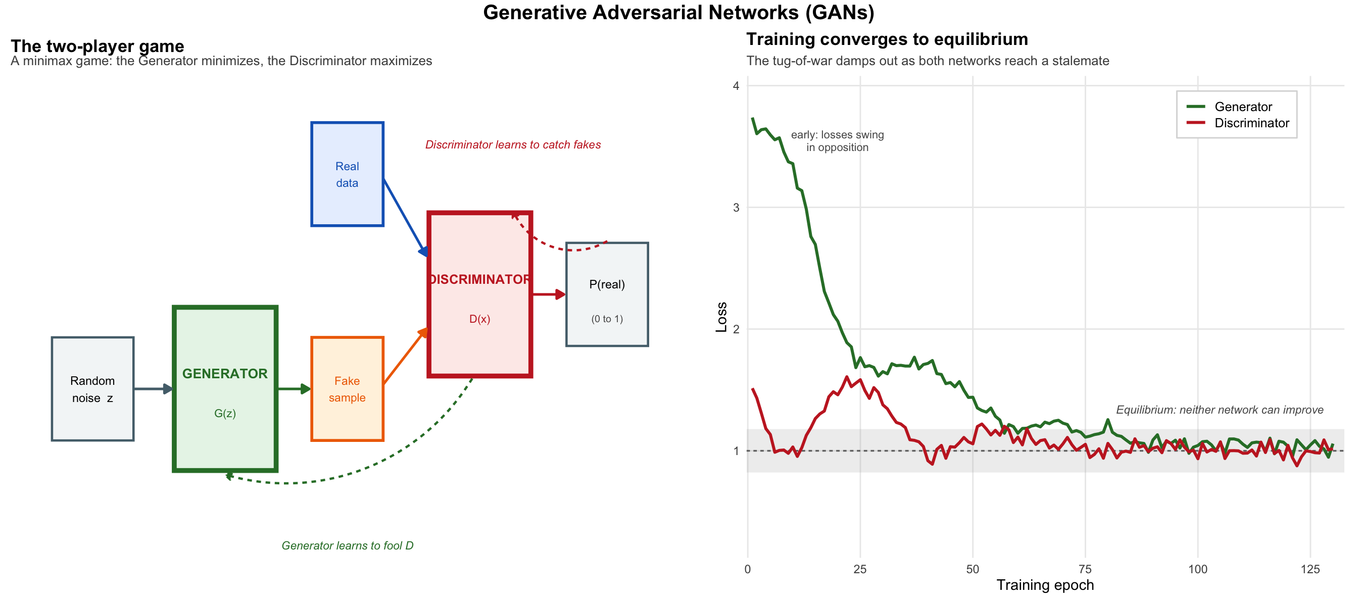
GANs: A minimax game where the Generator learns to fool the Discriminator, while the Discriminator learns to spot fakes. This adversarial training produces remarkably realistic synthetic data.

In 2014, Ian Goodfellow, then a PhD student, invented Generative Adversarial Networks (GANs). This was a novel approach to training generative models, pitting a Generator (which creates fake images) against a Discriminator (which tries to spot the fakes) in a minimax game. The result was a marked improvement in the realism of AI-generated images.

Architectural Innovations (2014-2017)

The years following AlexNet saw rapid experimentation with network architectures, each addressing specific limitations of previous designs.

VGGNet, developed at Oxford in 2014 by Karen Simonyan and Andrew Zisserman, demonstrated that architectural simplicity could be effective. Using only 3×3 convolutional filters stacked to depths of 16-19 layers, VGG showed that very deep networks with small filters could achieve excellent performance. The architecture achieved 7.3% error on ImageNet while being conceptually straightforward.

GoogLeNet (also called Inception), developed by Google in 2014, took a different approach. Christian Szegedy’s team introduced “Inception modules” that computed multiple convolution sizes (1×1, 3×3, 5×5) in parallel, allowing the network to capture features at different scales simultaneously. This architecture reached 22 layers deep while using 12 times fewer parameters than AlexNet, winning the 2014 ILSVRC with 6.7% error.

ResNet, introduced by Kaiming He and colleagues at Microsoft Research in 2015, solved the degradation problem in very deep networks through skip connections. By adding the input of a layer directly to its output, gradients could flow unimpeded through the network. This simple modification enabled training of networks with 152 layers that achieved 3.57% error on ImageNet, edging past the 5.1% error of a single trained human annotator on the same benchmark.

DenseNet, proposed in 2017, extended the skip connection idea by connecting each layer to all subsequent layers. This dense connectivity pattern promoted feature reuse and gradient flow while requiring fewer parameters than comparable architectures.

Architecture was only half the story of these years. The same period produced training methods that made deeper networks practical to fit. Kingma and Ba’s Adam optimizer (2015) gave each parameter its own self-adjusting learning rate, which removed much of the hand-tuning earlier methods demanded. Batch normalization (Ioffe and Szegedy, 2015) renormalized the inputs to each layer as training progressed, letting very deep networks converge faster and more reliably - though later work by Santurkar and colleagues showed the original “internal covariate shift” story was largely wrong, and the real benefit is a smoother loss landscape. Augmentation grew more inventive too: beyond the random crops and flips AlexNet already leaned on, Cutout and Mixup showed that even deliberately corrupted or blended training images could improve how well a model generalized.

The Representation Learning Revolution

When researchers looked inside trained networks, they found something interesting. Early layers learned simple features (edges, colors). Middle layers combined these into parts (eyes, wheels). Deep layers represented complete concepts (faces, cars).

The network had discovered the hierarchical structure of the visual world - without being told it existed.

This suggested an important principle: intelligence might emerge from learning good representations of the world.

Part VI: Transformers and the Scaling Bet (2017-2020)

Where we areThe unifying idea. A layer that lets every word weigh every other word replaces specialized designs for text, images, and sound. Making it larger keeps working, and that becomes the field's investment thesis.

Sequential models faced inherent limitations with long-range dependencies and contextual reasoning. The Winograd Schema Challenge illustrated this problem: resolving the pronoun “it” in “The animal didn’t cross the street because it was too tired” versus “The animal didn’t cross the street because it was too wide” requires understanding semantics and world knowledge, not just syntax. Recurrent Neural Networks, even with LSTM gates, struggled with such relationships as information had to pass through many sequential steps.

RNNs processed text one word at a time, maintaining a hidden state that theoretically captured all previous context. In practice, this sequential processing created an information bottleneck. CNNs could process multiple positions simultaneously but were limited to local receptive fields. The alternative was to allow every position in a sequence to directly attend to every other position.

Attention Is All You Need (2017)

From attention to a working GPT

The best visual explanation of attention I have found is Grant's chapter 6: how each token looks at the others through queries, keys, and values. I have put the conceptual takes first and the build-it-yourself takes last, because the idea lands hardest in that order. Karpathy's video is where you stop reading about attention and watch a working GPT get assembled from scratch, and Kilcher's walkthrough of the original paper is the bridge back to the 2017 source.

In June 2017, Vaswani et al. from Google Brain published “Attention Is All You Need”, introducing the Transformer architecture. The paper demonstrated that attention mechanisms alone, without recurrence or convolution, could achieve state-of-the-art results in machine translation.

Understanding Attention: The Core Innovation

The Problem: How can we let every position in a sequence directly interact with every other position, without stepping through the sequence one token at a time?

The Solution: Attention mechanisms compute a weighted average of all positions, where the weights are learned based on content similarity.

Before the formalism, it helps to follow a single word through the machinery. Take the sentence “The cat sat on the mat” and stand at the word “sat”. Right now “sat” is just a generic embedding of the verb, the same vector it would have in any sentence. To become useful it needs to know who did the sitting and where. So “sat” broadcasts a question to the rest of the sentence: something like “who is my subject, and what surface is involved?” That question is its query vector - not a sentence in English, of course, but a direction in a learned vector space that the model has discovered is a good way to ask for subjects and locations.

Every other word in the sentence, “sat” included, has already advertised what it can answer. Each one carries a key vector, which works like a label on a filing drawer: “I am a concrete animate noun”, “I am a preposition introducing a location”, “I am a determiner and mostly uninformative”. The model compares the query from “sat” against each of those labels with a dot product, and the size of the match becomes a raw score. Softmax turns those scores into a set of weights that sum to one, so the comparison stops being an absolute judgment and becomes a budget: out of all my attention, how much goes to each word? For “sat” in this sentence, most of that budget lands on “cat” and on “sat” itself, a little on “on”, and almost nothing on the two instances of “the”.

The last step is where the content actually moves. Alongside its key, each word carries a value vector, which is the information it is willing to hand over if attended to. The output for “sat” is the weighted average of all six value vectors, weighted by that attention budget. What comes out is no longer the generic verb “sat” - it is a version of “sat” that has absorbed a good deal of “cat” and a bit of “on”. Do this for every word at once and you get a whole new set of representations, each one recolored by whichever other words mattered to it. That is the entire mechanism. The rest is bookkeeping. There is a clinical parallel I find genuinely useful here: the key is what a report says it contains, the value is the finding itself, and the query is the specific question you walked in with. The same slide answers different questions depending on who is asking.

The three panels below show the same idea at three zoom levels. In the top panel, follow the vertical columns: each token is projected into a key and a value, the query from “sat” is compared against every key to produce the raw scores, softmax turns those into the weight bars (note how the bar under “cat” and “sat” dominates), and the values are then blended in proportion to those bars to make the output. In the middle panel, the row-by-row structure is the point: each row is one word’s attention budget, and every row sums to 1.00, so you are looking at all six words doing simultaneously what the first panel showed for one. The “sat” row of that heatmap is exactly the weight vector from the panel above it. In the bottom panel, notice that the same six tokens appear three times with different arcs drawn over them: one head has learned to link a verb to its subject, another mostly looks at immediate neighbors, and a third reaches across the sentence to tie an entity to a location. These are not sequential stages - they run side by side, and their outputs are concatenated at the end.

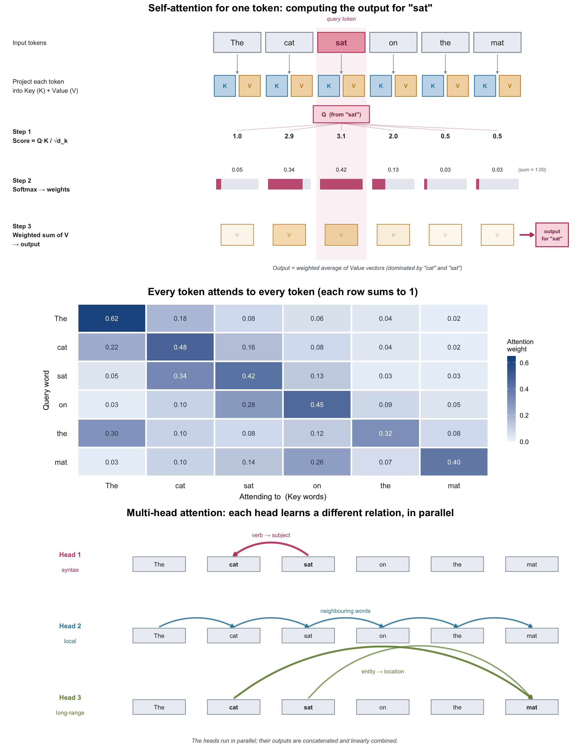
The Mathematics of Attention

The attention mechanism computes three learned linear projections for each input:

\[\text{Attention}(Q, K, V) = \text{softmax}\left(\frac{QK^T}{\sqrt{d_k}}\right)V\]

Where: - Q (Query): What information am I looking for? (What does “cat” need to know?) - K (Key): What information do I contain? (What can each word provide?) - V (Value): The actual information to aggregate (The content to use) - $\sqrt{d_k}$: Scaling factor that keeps dot products from growing so large that softmax saturates into near-one-hot weights

Why This Works:

The reason this beat recurrence is worth stating plainly, because it is mostly about distance and about hardware. In an RNN, information from word 1 reaches word 30 only by being carried through twenty-nine intermediate hidden states, and anything that survives that chain has been repeatedly overwritten along the way. In attention, word 30 queries word 1 directly - one comparison, one step, no matter how far apart they sit. That is the first half. The second half is that because no position depends on the previous position’s output, every position’s query, key, and value can be computed at the same time, so a whole sequence becomes one large matrix multiplication instead of a loop with hundreds of iterations. An RNN leaves most of a GPU idle waiting on the previous timestep; a Transformer saturates it. Layered on top of both properties is the fact that the weights are learned rather than fixed, so the model discovers for itself what is worth attending to for a given task, and multi-head attention lets it track several different kinds of relationship at once rather than collapsing them into a single notion of relevance.

The Transformer Architecture

Self-attention as described so far is one component, and on its own it is not enough to build a working model. The Transformer surrounds it with a few pieces, each solving a specific problem.

Multi-head attention runs several attention operations side by side instead of one. A single set of query and key projections can only encode one notion of “relevant”, and language needs more than one at a time: agreement between a verb and its subject, the referent of a pronoun, and the tone of a nearby adjective are all real relationships that a single head would have to compromise between. Splitting the representation across heads lets each learn its own kind of relationship, and their outputs are concatenated and mixed back together at the end.

Positional encodings exist because attention, as constructed, is order-blind. Shuffle the input words and every query-key comparison returns exactly the same value, so “the cat sat on the mat” and “the mat sat on the cat” would be indistinguishable. Since order carries no weight in the mechanism itself, position has to be injected into the input directly; the original paper does this by adding sinusoidal position signals to the embeddings so that a token’s representation encodes both what it is and where it sits.

Residual connections and layer normalization are what make a deep stack of these blocks trainable at all. This is the same lesson as ResNet earlier in this essay: let each block learn a modification to its input rather than a wholesale replacement, and add that modification back to what came in, so gradients have a short path down through the network no matter how many layers are stacked. Layer normalization keeps the scale of activations stable as they pass through those repeated additions, which in practice is the difference between a deep model that converges and one that does not.

Feed-forward networks are where per-token processing happens. Attention moves information between positions but is, at its core, a weighted average - a linear operation on the values. The feed-forward block that follows each attention layer operates on each token independently and adds the non-linear transformation, giving the model somewhere to actually process what it just gathered before passing it up to the next layer.

This architecture enabled a new paradigm: massive self-supervised pre-training followed by task-specific fine-tuning.

ELMo: Deep Contextualized Word Representations

Peters et al. (2018) from Allen AI showed that deep, bidirectional language models could learn rich word representations. Unlike Word2Vec’s static embeddings, ELMo created different representations for “bank” in “river bank” vs “bank account.”

GPT-1: Unsupervised Pre-training

OpenAI’s GPT (June 2018) used a Transformer decoder to predict the next word on BookCorpus (7,000 unpublished books). The key insight: unsupervised pre-training followed by supervised fine-tuning significantly improved performance on downstream tasks.

BERT: Bidirectional Understanding

Google’s BERT (October 2018) introduced a breakthrough: Masked Language Modeling (MLM).

The Problem: GPT could only read left-to-right. But language has bidirectional context.

The Solution:

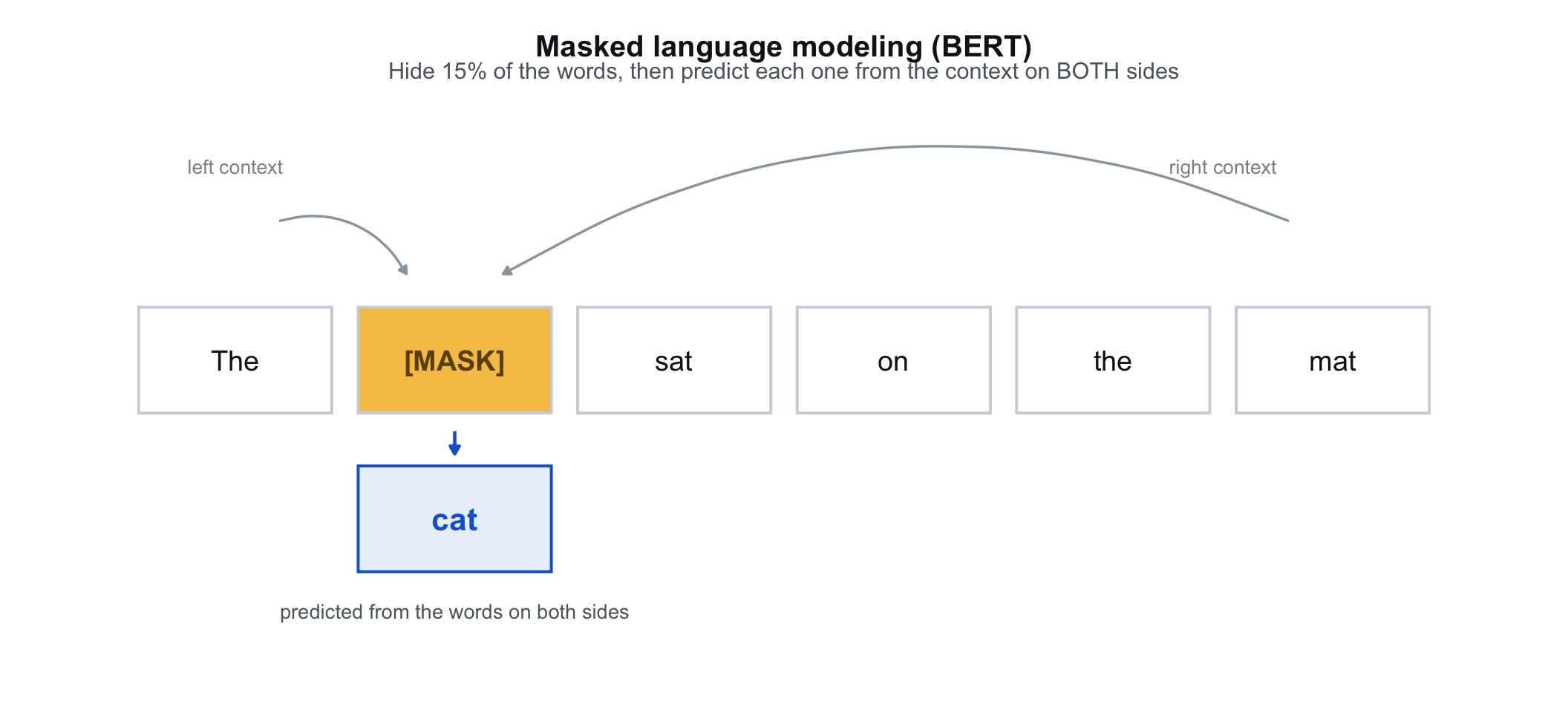
Masked language modeling: BERT learns by predicting randomly masked words from bidirectional context, creating rich representations without labeled data.

Randomly mask 15% of tokens
Predict masked tokens from bidirectional context
80% of time: replace with [MASK]
10% of time: replace with random token
10% of time: keep unchanged

This forces the model to: - Use bidirectional context (can’t just copy) - Be robust to noise (random replacements) - Maintain distributional consistency (unchanged tokens)

Results: BERT achieved SOTA on 11 NLP tasks. More importantly, it learned rich representations that could be fine-tuned for any task with minimal data.

The Scaling Hypothesis (2019-2020)

How LLMs learn and scale

This is the part I found hardest to get an honest picture of: what pretraining actually optimizes, and why making the model bigger kept working. Cross-entropy is the loss doing all the work, and Grant's 2026 compression series is the clearest argument I have seen for why a better language model is literally a better compressor. Karpathy's deep dive is the single best plain-English tour of how these systems are built, trained, and fine-tuned.

While Google focused on architecture improvements, OpenAI bet on scale. Their GPT series just predicted the next word - but did it on massive amounts of text with increasingly large models:

GPT-1 (2018): 117M parameters, 4.5GB of text
GPT-2 (2019): 1.5B parameters, 40GB of text (WebText)
GPT-3 (2020): 175B parameters, 570GB of text (CommonCrawl + books + Wikipedia)

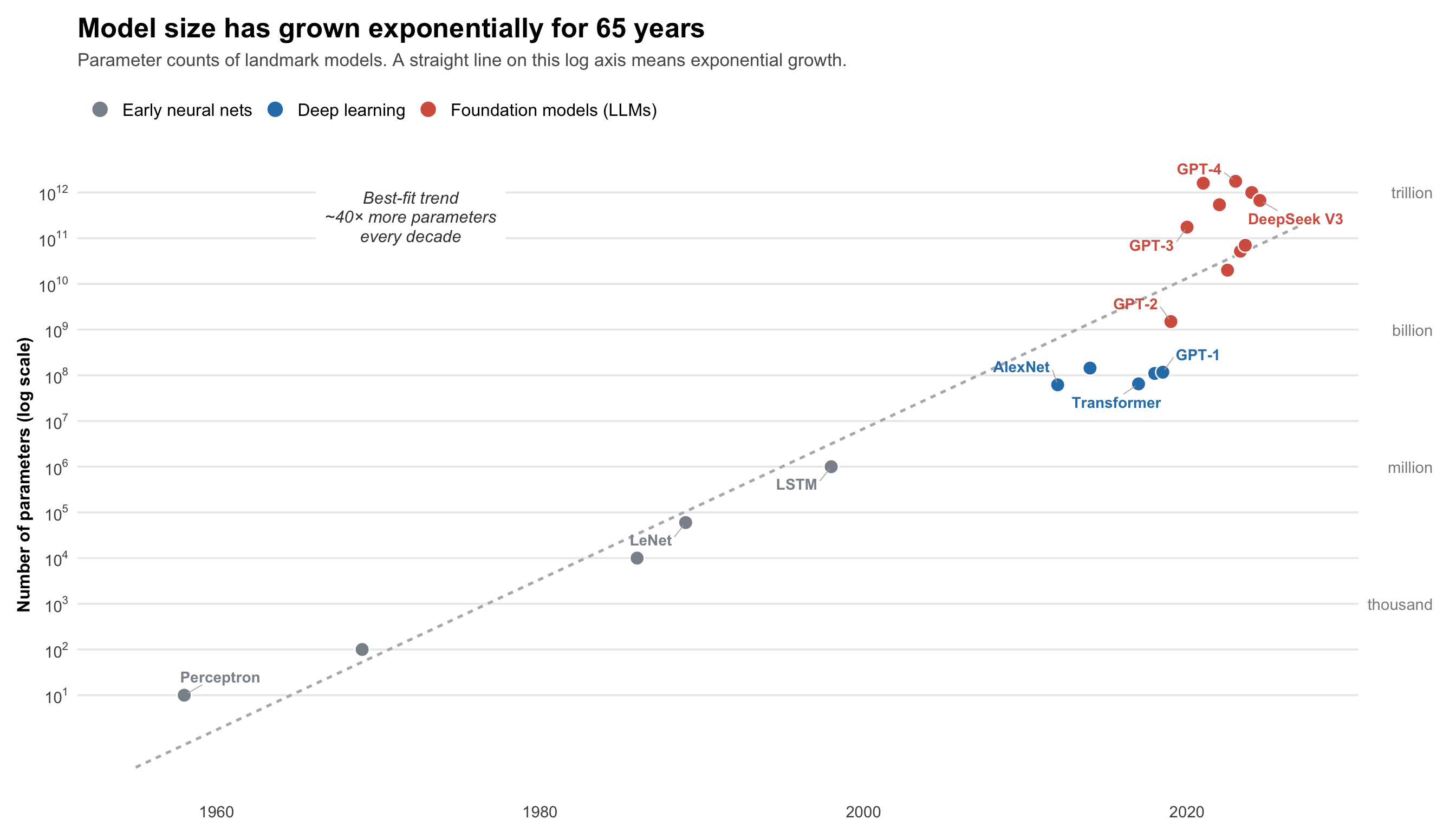
Model size has grown in distinct phases: slow growth in the classical AI era, steady increase during deep learning, and rapid scaling in recent years. GPT-4’s leaked/estimated 1.76 trillion parameters would have seemed unlikely just 5 years earlier.

GPT-2: A Staged Release

In February 2019, OpenAI announced GPT-2 with unusual fanfare - and controversy. They initially refused to release the full model, citing concerns about malicious use. The 1.5B parameter model could generate coherent, multi-paragraph text that was often indistinguishable from human writing.

GPT-3: Emergent Abilities

GPT-3’s training gives a sense of the scale involved: - Cost: ~$4.6 million in compute - Training time: 34 days on 10,000 V100 GPUs - Energy: 1,287 MWh (enough to power 120 US homes for a year) - Data: 300 billion tokens (roughly 225 billion words) - Architecture: 96 layers, 96 attention heads, 12,288 dimensional states

The model exhibited emergent abilities that weren’t explicitly programmed: - Three-digit arithmetic: absent in smaller models, reliable only in the larger ones - Analogical reasoning: emerged only at larger scale
- Code generation: appeared only in the largest models - Few-shot learning: Could learn new tasks from 1-10 examples

Most remarkably, GPT-3 showed in-context learning - it could learn new patterns during inference without updating weights. Show it a few examples of English→French translation, and it would translate. Show it math problems with solutions, and it would solve new ones.

The Scaling Laws: Kaplan et al. (2020) discovered predictable relationships:

Loss = A / (N^α × D^β × C^γ)

Where N = parameters, D = data, C = compute. Performance improved predictably with scale - until emergent capabilities appeared suddenly, like phase transitions.

The model had learned to perform complex reasoning tasks simply by predicting the next word in internet text. This raised an interesting question: how much of intelligence emerges from pattern recognition at sufficient scale?

Part VII: Large Language Models as Products (2021-Present)

Where we areThe consequences. Research prototypes ship as tools that write code, draft documents, and read medical images. The hard questions turn to compute cost, who gets access, and how behavior is steered.

The scaling hypothesis - initially dismissed as brute force engineering - turned out to reveal something important. Beyond certain thresholds of scale, new capabilities appear discontinuously. These aren’t incremental improvements but something more like phase transitions: capabilities such as arithmetic, multi-step reasoning, and inference about others’ mental states tend to appear only past certain scales, though the exact thresholds are fuzzy and depend on the model and task. It’s still not clear exactly why this happens - and it’s worth noting the finding is contested: Schaeffer and colleagues argued in 2023 that much of the apparent suddenness is an artifact of discontinuous metrics like exact-match accuracy, and that smoother metrics show more gradual gains.

GPT-3 was trained to predict the next word. That’s it. But somewhere around 175 billion parameters, it learned to code, translate languages it was never explicitly taught, solve math problems, and write poetry. This is what the field came to call emergence - quantity turning into quality - though as the caveat above notes, how sudden those jumps really are depends partly on how you measure them.

A Wave of Foundation Models

Post-GPT-3, AI development exploded. Every major tech company and dozens of startups raced to build foundation models.

Multimodal Intelligence (2021-2022)

The success of transformers in language raised an uncomfortable question for computer vision researchers: Were CNNs actually necessary? For a decade, convolutional neural networks had dominated vision tasks. Their architecture encoded a powerful assumption - that visual features are local and hierarchical. Edges combine into textures, textures into parts, parts into objects.

The question was whether that assumption was limiting performance.

Vision Transformers

Patches, prompts, and pixels

The jump from language to images is where the transformer stopped being a text architecture and became a general one. These start with the two papers that did it (Kilcher walks through ViT and CLIP at a comfortable pace) and then move to diffusion, which is a genuinely different idea: add noise to an image step by step, then train a network to run the process backwards. Mike Pound's pair is the best mechanical explanation, right down to the code.

Alexey Dosovitskiy’s team at Google Brain tried something that seemed overly simple: chopping up images into squares and feeding them to a transformer like words.

Images aren’t text - they lack grammar, syntax, and sequential structure. A patch of blue pixels could be sky, water, or a shirt. Context matters differently than in language.

But when they trained their Vision Transformer (ViT) on 14 million images, it worked - and beat CNNs when given enough data. The key insight: spatial relationships in images can be modeled as sequences.

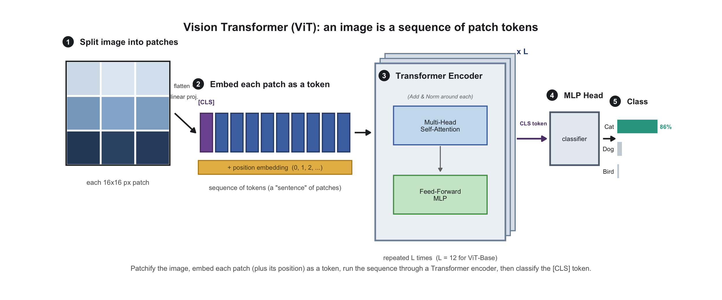
Vision Transformer splits images into patches, treating them as sequences similar to words in NLP, enabling powerful transfer learning from language models.

This approach succeeds because images contain long-range dependencies - features in one part of an image often relate to features in distant parts. While convolutional networks build up receptive fields gradually through layers, transformers can immediately attend to any patch from any other patch, capturing global relationships from the first layer.

Masked Image Modeling: Self-Supervised Learning for Vision

In November 2021, Kaiming He and his team at Facebook AI Research applied BERT’s masked language modeling approach to computer vision. Their Masked Autoencoders (MAE) trained vision models by randomly masking 75% of an image’s patches and training the model to reconstruct the missing regions.

This high masking ratio - much higher than the 15% typically used in language models - forced the model to understand global image structure rather than simply interpolating from nearby patches. Models trained this way learned comprehensive visual representations: they captured object structure, lighting patterns, texture continuity, and spatial relationships without requiring labeled data.

CLIP: Connecting Vision and Language

In January 2021, OpenAI introduced CLIP (Contrastive Language-Image Pre-training), which learned visual concepts from natural language supervision. Rather than training on manually labeled datasets, CLIP used 400 million image-text pairs collected from the internet.

The training approach used contrastive learning: given a batch of images and their corresponding text descriptions, the model learned to encode both modalities such that matched pairs had high similarity while unmatched pairs had low similarity. The vision encoder (either a ResNet or Vision Transformer) and text encoder (a Transformer) were trained jointly to project both modalities into a shared embedding space.

This approach enabled zero-shot transfer to downstream tasks. Without any task-specific training, CLIP achieved 76% accuracy on ImageNet classification - comparable to a ResNet-50 trained specifically on ImageNet. The model could classify images by comparing their embeddings to text embeddings of class descriptions like “a photo of a [class name].”

CLIP demonstrated that visual representations could be learned from natural language supervision at scale. The shared embedding space it created, where visual and textual concepts were aligned, became foundational for subsequent developments in text-to-image generation, visual question answering, and multimodal understanding.

Diffusion Models: A New Approach to Generation

Diffusion models introduced a fundamentally different approach to image generation. Rather than learning to generate images directly, they learned to reverse a gradual noising process. Starting with a clean image, the forward process progressively adds Gaussian noise over many steps until the image becomes pure noise. The model then learns to reverse this process, denoising step by step to recover the original image.

Stable Diffusion, released by Stability AI in 2022, made this approach practical for widespread use. By operating in a compressed latent space (typically 64×64) rather than pixel space (512×512), it reduced computational requirements by roughly 50x. Text conditioning was achieved through cross-attention layers that incorporated CLIP text embeddings at multiple scales throughout the denoising network. This architecture enabled high-quality text-to-image generation on consumer GPUs with 8GB of VRAM, democratizing access to powerful generative models.

ChatGPT and the Transformation of AI Interaction (November 2022)

On November 30, 2022, OpenAI released ChatGPT as a research preview. The model itself - a fine-tuned version of GPT-3.5 - wasn’t dramatically more capable than previous releases. What changed was the interface and training approach.

ChatGPT reached a million users in five days and a hundred million within two months, the fastest a consumer product had ever spread to that point.

The Role of Reinforcement Learning from Human Feedback (RLHF)

StatQuest walks through the three steps that turn a raw language model into a helpful assistant: collect human preferences, train a reward model, then fine-tune against it.

ChatGPT’s key innovation was the systematic application of Reinforcement Learning from Human Feedback (RLHF) to align the model with human preferences. The process involved three phases:

First, supervised fine-tuning created an initial instruction-following model. Human contractors wrote high-quality responses to thousands of diverse prompts, covering creative writing, coding, factual questions, and ethical scenarios. This dataset trained the base GPT-3.5 model to follow instructions rather than simply complete text.

Second, a reward model was trained to predict human preferences. Contractors ranked multiple model outputs for each prompt, typically comparing 4-9 responses. These rankings trained a 6-billion parameter model to score outputs based on helpfulness, harmlessness, and honesty - the three H’s that became OpenAI’s alignment targets.

Third, Proximal Policy Optimization (PPO) fine-tuned the language model to maximize the reward model’s scores while maintaining similarity to the original model through KL divergence penalties. This constraint prevented the model from finding adversarial solutions that gamed the reward function while producing nonsensical outputs.

The interface mattered. The chat format made AI feel like a collaborator rather than a tool. You could iterate, clarify, and push back.

The conversation shifted from “AI can’t do my job” to “what parts of my job can AI do?”

What 2023 Actually Changed

ChatGPT proved the demand; 2023 was the year the field worked out what to build in response. Three things shifted, and none of them are captured well by a list of release dates.

Frontier capability became legible

GPT-4 was the moment broad, professional-level competence stopped being a claim and became something you could measure. The clearest example was the bar exam, where the model moved from roughly the 10th percentile to the 90th - the same test, a different order of capability. Getting there was not subtle: training reportedly ran on an estimated 25,000 A100 GPUs over several months. What made this land was less any single benchmark than the breadth. A tool that could write, code, analyze, and reason at once forced a more honest question than “can AI do my job?” - namely, which parts of the work were ever the hard parts.

Anthropic released Claude into the same moment, but the interesting difference was in how the model was aligned rather than in a scoreboard. Their approach, Constitutional AI, worked roughly like this:

Train a helpful, harmless, honest assistant
Use AI feedback, not just human labels, to identify problematic outputs
Train the model to critique and revise its own responses
Result: a model that self-censors without explicit filters

The bet was that you could get a model to internalize a set of principles and hold itself to them, instead of bolting a filter onto the front. That is a different theory of how you make these systems safe, and it is worth noticing that the two leading labs disagreed about method this early.

The closed-versus-open split

The other durable division of 2023 was whether model weights should be open at all. Most labs sold access to their models through an API. Meta went the other way and released Llama 2 for free download, in sizes from 7 to 70 billion parameters, small enough that the 7B version ran on a decent laptop and the 70B approached the previous generation’s quality on a single GPU.

Open weights changed who could build. Within days of the release, researchers were fine-tuning variants for specific tasks; within months, hundreds of them existed. You no longer needed a lab’s permission or its billing to adapt a capable model to your own problem. The framing at the time was that Meta wanted to be the Linux of AI - to make its stack the shared infrastructure everyone built on, rather than depend on a competitor’s. Whatever the motive, the effect was that a large chunk of the field’s experimentation moved out of a handful of companies and into the open.

Efficiency and architecture

The third shift was about doing more with less compute, and Mistral’s Mixtral was the clearest case. It used a sparse Mixture of Experts design: 47 billion parameters in total, but only about 13 billion active for any given token. The result matched the previous generation’s quality at a fraction of the compute and ran on hardware that could not have held a dense model of comparable strength.

The idea underneath is simple once stated - not every token needs every parameter, so route each token to the few experts suited to it. It is an old idea, going back to Hinton in 1991, that finally became practical at scale.

The same year quietly settled the context-window race. Over 2023 the amount of text a model could hold at once grew by more than an order of magnitude - GPT-4 climbing from 8K toward 128K tokens, Claude reaching 100K, enough to read a novel like The Great Gatsby in a single pass. That turned out to matter less as a specification than as a change in what you could hand a model: a whole contract, an entire codebase, a full paper, rather than fragments you had to stitch together yourself.

Beyond Text (2024)

By 2024 the interesting frontier was no longer any single modality but the seams between them - what happens when a model treats speech, video, and physical action as things to be understood rather than transcribed into text first.

Voice without a text detour

The older way to build a talking assistant was a pipeline: transcribe your speech to text, feed the text to a language model, synthesize the reply back into audio. Every stage threw something away. Tone, hesitation, the exact moment you started to interrupt - all of it collapsed into a flat string somewhere in the middle.

The shift that mattered in 2024 was speech-to-speech models that skip the text intermediary entirely. The model hears audio and speaks audio, operating on sound directly, so prosody, timing, and emotion survive the round trip instead of being reconstructed from a transcript. Response latency dropped to roughly a quarter of a second, close enough to human conversational tempo that interruption and back-and-forth start to feel natural rather than walkie-talkie. The tradeoff is that continuous listening means continuous streaming to a server, which is a real privacy question and not a solved one.

Video and the physics question

Video generation raised a genuinely interesting question rather than just a better demo. Systems like Sora could produce a full minute of coherent footage - objects staying put when they moved off-screen, shadows tracking their light sources, glass shattering in roughly the right way - without anyone programming those rules in. Physics seemed to fall out of watching enough video.

The open debate is whether that counts as understanding. Does the model hold something like an internal model of how the world behaves, or has it pattern-matched enough footage that the statistically likely next frame usually happens to obey physics? The failure cases - liquids that briefly flow uphill, limbs that pass through solid objects - suggest the latter, or at least something short of a real world-model. It is an unresolved and clarifying question, because it is the same one we keep asking about these models in every other domain. Practically, the tools found early use in film previsualization, letting directors sketch shots before committing to production.

Embodiment and Moravec’s Paradox

The hardest problems turned out to be the ones a toddler solves without thinking. Pairing language models with robots let a machine take a spoken instruction, reason about what its cameras saw, and drive its actuators toward the goal, and by 2024 these systems could learn manipulation tasks from demonstration rather than hand-written code. But the frontier was not abstract reasoning - it was standing up, walking across an uneven floor, and closing a hand around an object without crushing it.

This is Moravec’s Paradox, and it remains the durable idea in this whole thread. High-level reasoning is cheap to compute; the sensorimotor skills we share with every animal are expensive, because evolution spent hundreds of millions of years tuning them and almost no time at all on chess. AI mastered the board game decades before it could reliably manage the walk to the table.

Code: from autocomplete to agents

The same year, coding assistants crossed from finishing your current line to attempting whole tasks on their own - reading an issue, editing across files, running the tests, and iterating. The honest measure of how far that had come is SWE-bench, which asks a system to resolve real GitHub issues. An early autonomous agent, Devin, resolved about 13.86% of them, against roughly 1.74% for a bare GPT-4 and the 20-30% a human junior developer manages. That is a real jump and still well short of a person. The pattern the numbers point to is augmentation, not replacement: the engineer moves toward architecture, requirements, and review while the model absorbs more of the implementation. The same generality showed up in vision, where promptable segmentation models learned to isolate any object in an image from a click or a box, with no task-specific retraining.

The Competition Intensifies (2024)

By late 2024 the frontier was crowded in every direction at once: the most capable models, the cheapest, the fastest, and the most open were four different systems from four different labs. One chart tells that story better than any release list.

The Reasoning Turn (Late 2024)

Spending Compute at Inference

For most of the past decade, the recipe for a better model was to train a bigger one. Late in 2024, OpenAI’s o1 and o3 pointed at a second axis. Rather than front-loading all the compute into training, these models spend it at inference, working through a problem step by step before answering. Easy questions get quick replies; hard ones trigger extended chains of thought that consume orders of magnitude more compute, and because the model exposes its reasoning, its mistakes become legible rather than hidden inside a single opaque guess.

The result that caught my eye was ARC-AGI, a benchmark of abstract visual puzzles built to resist memorization. o3 scored 87.5%, the first time a system crossed the roughly 85% average for humans. Its creator, François Chollet, was quick to caution that this did not mean the model had reached general intelligence. The caveat matters partly because of the price: reaching that score cost on the order of $3,700 of compute per task. Whether that trade of dollars for reasoning holds up is one of the things I am watching.

Frontier Capability at a Fraction of the Cost

While one lab spent more to think longer, a team in Hangzhou showed how much could be done with less. DeepSeek reported training its V3 model for about $5.57 million, against the roughly $100 million widely estimated for GPT-4, and released the weights openly.

The efficiency came from stacking careful engineering rather than any single trick. A Mixture-of-Experts design activates only 37 billion of the model’s 671 billion parameters for any given token, so most of the network sits idle on each step. FP8 mixed-precision training roughly halves the memory footprint by holding weights in eight bits while keeping the sensitive computations at higher precision. And a multi-token prediction objective has the model predict one extra token beyond the immediate next one during training, which sharpens its sense of planning and, at inference, supports a decoding scheme that runs on the order of 1.8 times faster. The lesson I take from it is a simple one, worth stating once: determined engineering can rival the frontier labs at a fraction of the reported cost.

These two threads, thinking longer and doing more with less, pulled in opposite directions on cost while both pushing capability forward. They are much of the ground on which 2025 would be built.

2025 and 2026: Reasoning, Agents, and Cost

Where we areThe unfinished part. Models spend more compute before answering, systems run for hours unattended, and evaluation cannot keep up. What follows is a record of an argument still in progress.

I am writing this in the middle of 2026, which means everything in this section comes with a caveat: it is too early to know which of these developments will still look important in a few years and which were noise. The o3 announcement that closes the section above was only the start of a strange, fast stretch. Let me try to trace three threads through it, continuing the two the reasoning turn opened.

The first is that reasoning went open and cheap almost as soon as it arrived. Within weeks of o3 being announced, a team released DeepSeek R1, an openly available model that reasoned in much the same o1-class way, with the weights there for anyone to download and run. The step-by-step reasoning that had looked like a proprietary frontier capability was, suddenly, a commodity. And the efficiency trend the V3 story hinted at kept compounding through the open-weight releases that followed, so that the striking thing was no longer that an open-weight lab could reach the frontier but how little compute it took to get there.

The second thread is that the frontier kept moving, but the shape of the story changed. GPT-5 and Gemini 3 arrived to a lot of anticipation, and they were genuinely stronger, but they felt more like consolidation than revolution: the curve bending upward rather than snapping. The real shift was quieter and harder to benchmark. Models stopped only answering and started acting. They browsed, wrote and ran code across many files, called tools, and carried a task through several steps without a human at each turn. That move from a system that responds to one that does multi-step work is, I think, the part of this period that will read as the actual break.

The third thread is that some benchmarks fell and others held. Systems reached gold-medal-level performance on olympiad mathematics, a result that a decade ago would have been the headline of the year. But ARC-AGI-2, built specifically to resist them, has not been cleared: the best verified systems sit under forty percent on it while people score near the ceiling. And yet I want to be honest about what they do and do not tell us, because this is familiar ground for me. In medicine we have always known that passing the boards and being good at the bedside are different things, and they come apart in both directions. Benchmark-passing and general competence keep drifting apart the same way. A model can prove a hard theorem and still fumble a task a careful person would not.

That gap is exactly why this is the place to stop narrating and start reflecting. The dates and model names will keep coming, faster than any essay can catch. What is worth sitting with is not the next number but the patterns underneath all of it, and those are old.

Some Closing Thoughts

If the “we built it before we understood it” theme lands for you, this Welch Labs essay sits with the deepest open question: why do these enormous models generalize at all, instead of just memorizing?

A few patterns came up repeatedly in this history:

The simplest solutions kept winning. Backpropagation is just the chain rule. Attention is weighted averaging. ReLU is max(0,x). The ideas that changed everything were often embarrassingly simple in hindsight.
Scale beat cleverness. Every time we tried to encode human knowledge directly - expert systems, hand-crafted features, symbolic reasoning - learning from data at scale won. Rich Sutton called this the “bitter lesson.”
We built before we understood. We could fly before we understood aerodynamics. We’re building capable AI systems before we fully understand intelligence. That’s how a lot of progress actually happens.
Progress came in jumps. The Perceptron’s death, AlexNet’s breakthrough, ChatGPT’s launch - the field advanced through discontinuous leaps rather than gradual improvement.

After going through this history, what strikes me most is that we still don’t really understand why these systems work as well as they do. We can build them, train them, and deploy them, but the internal mechanisms remain largely opaque. A model with hundreds of billions of parameters can’t be easily simplified or explained.

I’ve certainly missed important developments and probably mischaracterized some things. The field moves fast, and parts of this are likely already outdated. But I hope it’s useful as an overview of how we got here.

The resources section below has papers and courses that go much deeper. The field is more accessible than ever - most important papers are freely available, and capable models can run on consumer hardware.

Thanks for reading.

Essential Resources

These are the papers I keep going back to, arranged the way the story ran. Most of the field’s landmarks are a free PDF away, which is one of the genuinely good things about this discipline.

If you want a starting path rather than a reading list, these eight get you from the first artificial neuron to the modern era, and you can read all of them in a week: McCulloch & Pitts (1943), Turing (1950), Rumelhart, Hinton & Williams (1986), LeCun et al. (1998), Hochreiter & Schmidhuber (1997), Krizhevsky et al. (2012), Vaswani et al. (2017), and Brown et al. (2020). Everything else below is depth on a particular thread.

Essential Papers in AI History

Foundational Works (1943-1969)

The Learning Revolution (1974-1998)

Statistical Learning (1995-2011)

Deep Learning Era (2012-2016)

Attention & Transformers (2014-2020)

Multimodal & Vision (2020-2022)

Diffusion Models & Generation (2020-2023)

Large Language Models & RLHF (2022-2024)

Where to Learn More

Visual & Interactive Learning

3Blue1Brown Neural Network Series: Grant Sanderson’s animated visual explanations
The Illustrated Transformer: Jay Alammar’s visual guide to transformers
Distill.pub: Interactive visualizations of ML concepts
Lil’Log: Lilian Weng’s comprehensive ML tutorials
The Annotated Transformer: Line-by-line implementation in PyTorch
CNN Explainer: Interactive CNN visualization
Transformer Explainer: Interactive transformer visualization
Seeing Theory: Visual introduction to probability and statistics
TensorFlow Playground: Interactive neural network in your browser
Understanding LSTM Networks: Chris Olah’s classic LSTM explanation
The Neural Network Zoo: Visual guide to neural architectures

University Courses (Free)

Stanford CS231n: Convolutional Neural Networks for Visual Recognition (Fei-Fei Li, Andrej Karpathy)
Stanford CS224n: Natural Language Processing with Deep Learning (Chris Manning)
MIT 6.034: Artificial Intelligence (Patrick Winston)
MIT 6.S191: Introduction to Deep Learning
Berkeley CS182: Deep Learning
Berkeley CS285: Deep Reinforcement Learning (Sergey Levine)
CMU 11-785: Introduction to Deep Learning
NYU Deep Learning: Yann LeCun and Alfredo Canziani
Fast.ai Practical Deep Learning: Top-down practical approach (Jeremy Howard)
DeepLearning.AI Specializations: Andrew Ng’s comprehensive courses
Full Stack Deep Learning: Production ML engineering
Harvard CS50 AI: Introduction to AI with Python

Books & Textbooks

Deep Learning by Goodfellow, Bengio, Courville: The definitive textbook (free online)
Pattern Recognition and Machine Learning by Bishop: Bayesian perspective (free PDF)
The Elements of Statistical Learning by Hastie, Tibshirani, Friedman: Statistical foundations (free PDF)
Dive into Deep Learning: Interactive book with code
Understanding Deep Learning by Simon Prince: Modern comprehensive text (2023, free)
Probabilistic Machine Learning by Kevin Murphy: Two-volume modern treatment
Speech and Language Processing by Jurafsky & Martin: NLP bible (free)
Reinforcement Learning: An Introduction by Sutton & Barto: RL classic (free)
Mathematics for Machine Learning by Deisenroth et al.: Mathematical foundations (free)
The Little Book of Deep Learning by François Fleuret: Concise introduction (free)
Neural Networks and Deep Learning by Michael Nielsen: Intuitive introduction (free)

Copyright & Citation

Citation: Pettit, R. W. (2026). AI: A Technical History. https://rowlandpettit.com/ai.html

Last updated July 2026.